Steering vectors estimate an average regression gradient

Here is a claim that sounds strange at first: when an engineer nudges a language model’s activations to make it write more positively, the nudge is, to a good approximation, an estimate of a regression slope. By activations we mean the vectors of numbers the model computes at each layer as it reads text; ours are read at layer 6 of GPT-2’s 12 blocks and averaged over each sentence’s tokens, so every sentence becomes one 768-dimensional vector. The regression behind the claim is concrete: regress the outcome, here a sentiment label, on the activation vector; at each data point the fitted surface has a slope vector that says which way to move the activation to raise the predicted outcome; average those slope vectors over the data. That average gradient is the same object that econometricians have been estimating since the average-derivative literature of the late 1980s. A steering vector is therefore a statistic, with sampling error and an estimand, and the usual questions apply: is there a better estimator? How much data does it need? When does sophistication stop paying?

We say “to a good approximation” deliberately; the test behind the hedge is specific. We compare two directions: the difference-in-means steering direction (the mean activation of the positive sentences minus the mean activation of the negative ones) and the regression-gradient direction of a linear probe (a simple classifier, here a logistic regression, trained on the frozen activations to predict the sentiment label; “the probe’s direction” is its coefficient vector). We measure their agreement by cosine similarity against a bar of 0.70 fixed before any analysis ran, in a local, timestamped working document locked on 2026-06-08 and included in the series’ replication repository (not an OSF or AsPredicted registration); we call it the advance document below. The observed cosine is 0.63, short of that bar; the body of this piece returns to the gap.

This is the second piece in a three-part series working through Avi Feller’s talk “Classical Statistics in the Age of AI” (Stanford Bay Area Tech Economics Seminar, June 4, 2026); his paper and code remain unpublished, so we implement the method described in his abstract ourselves. Part 1 tested his “do no harm” correction for AI-assisted estimation, and Part 3 asks whether a language model’s internal representations can out-predict a plain logistic regression on a real survey. The numbers are ours, on our toy setup; below we mark where the results matched the advance document’s predictions and where they did not.

What activation steering is

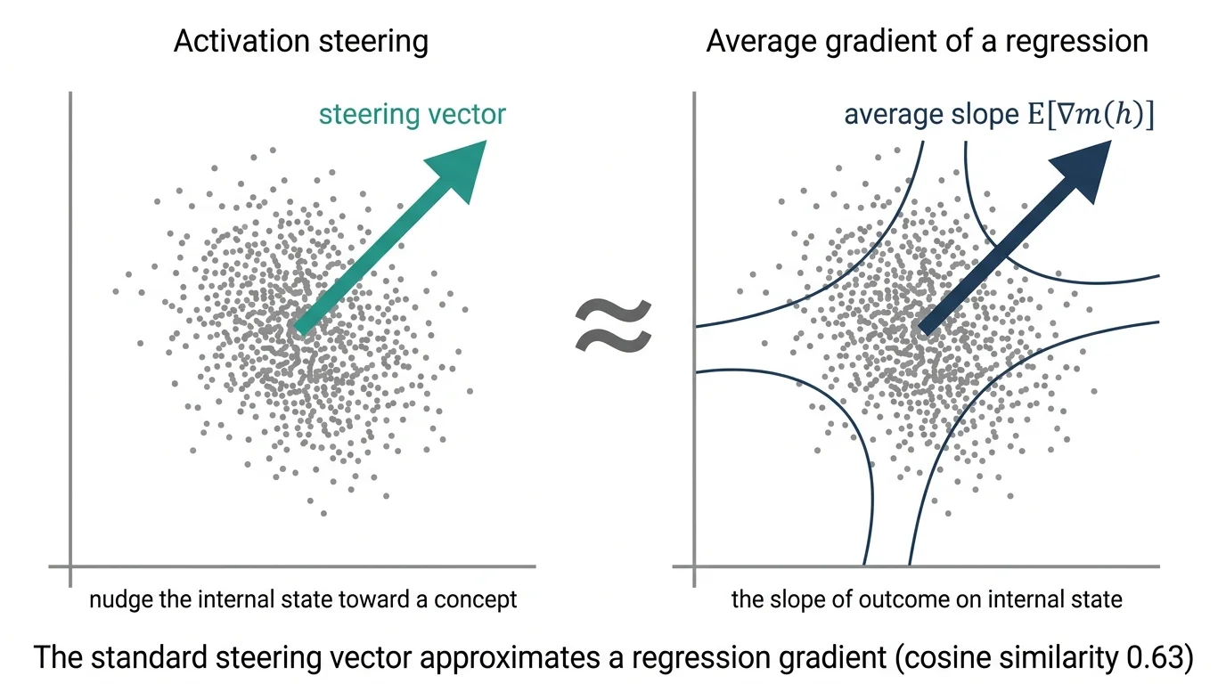
Activation steering means adding a fixed vector to a language model’s activations so that its output shifts in a chosen direction: more positive, more honest, more refusing. The recipe popularized in the activation-steering literature is simple: run a batch of positive examples through the model and record the activations; do the same for negative examples; subtract the two mean vectors; add the difference, scaled, at generation time, and the model’s tone moves.

To an economist, “subtract two group means” is the first estimator we ever learn, and that is Feller’s observation: the difference-in-means steering vector implicitly estimates the average gradient of the regression of sentiment on the activations. Average derivatives come with a well-developed menu of estimators, from the naive difference in means to estimators reaching the best possible variance among methods assuming no functional form.

Which suggests an experiment: if the nudge is a regression, a better regression estimator should produce a better nudge. Does it?

The setup

Everything runs on a laptop. The model is GPT-2 (124 million parameters), open weights, run locally, with activations read at layer 6 and mean-pooled as above. The construction corpus is roughly 400 short sentences generated from templates: 15 everyday subjects (“The meal”, “The movie”) crossed with 20 positive or 20 negative adjectives in 5 sentence templates, giving 200 positive and 200 negative sentences, held fixed throughout. The judge is DistilBERT fine-tuned on SST-2 (the Stanford Sentiment Treebank, a standard sentiment benchmark). The template sentences are not drawn from SST-2, so the judge never saw them or anything from their distribution in training; judge and corpus are independent.

The evaluation protocol is the same for every estimator. We take 8 fixed neutral prompts (“I went to the new restaurant downtown and”, “The weather today was”, and six more). For each direction, we add plus or minus K times the unit vector to the layer-6 activations during generation, where K is 5 percent of the typical activation length, and generate 30 tokens greedily. The judge scores each completion’s positive-class probability on a 0-to-1 scale. Separation is the mean score under positive steering minus the mean under negative steering; larger separation means the nudge moved the writing further.

For uncertainty we repeat everything across 25 seeds. One seed is one bootstrap resample, with replacement, of the 400 construction sentences; all four directions below are re-estimated on the resample, and the same 8 evaluation prompts are scored. The intervals quantify resampling variability of the construction set, on one model and one prompt set.

Does the nudge point where the regression points?

Mostly, with a caveat. The cosine similarity between the two directions, on a scale from -1 to 1, comes out at 0.63 [0.55, 0.71] over 25 seeds. That is well above what unrelated directions in a 768-dimensional space would show, so the data supports the basic claim: the engineering trick and the regression gradient point in broadly the same direction. But the advance document fixed 0.70 as the criterion for calling the two directions “the same object,” and 0.63 misses it, though the CI upper bound of 0.71 means the data do not statistically rule out meeting it. An earlier 5-seed run had recorded 0.749, which would have cleared the bar; the rerun overwrote its raw output, leaving the 0.749 only as a contemporaneous note in results.json, the results file published in the series’ replication repository, and the better-powered 25-seed estimate says that number was too high. We read this as directional support with a missed criterion: the nudge approximates the regression gradient, more loosely than the advance prediction said.

The estimator ladder

If steering is average-gradient estimation, the econometrics toolbox offers a ladder of estimators; we climb it rung by rung, measuring the steering effect at each step. Each rung produces one 768-dimensional direction, and all four are scaled to unit length and sign-aligned before steering, so every estimator is compared at the same magnitude and only the direction differs.

1. Raw difference-in-means. Subtract the mean activation of the negative sentences from the mean activation of the positive ones. The 768 entries of that difference are the direction. Separation: 0.755 [0.705, 0.804].

2. Probe gradient. Train an L2-regularized logistic regression on the 400 activations to predict the label; its coefficient vector is the direction. For a linear model the gradient of the fitted function is the coefficient vector, the same at every data point, so averaging gradients over the data returns the coefficients; a “probe direction” and a “regression gradient” are therefore the same object here by construction. Separation: 0.818 [0.771, 0.866].

3. Whitened difference-in-means. Compute the activation covariance matrix Sigma (with a small ridge for numerical stability) and solve Sigma times v equals (mu_pos minus mu_neg); the direction is v, Sigma-inverse times the raw difference. The adjustment stops correlated, high-variance coordinates from dominating the direction; it is the same move that distinguishes generalized least squares from ordinary least squares. Separation: 0.863 [0.823, 0.904].

4. Cross-fit orthogonal estimator. Built in four moves. First, compress the 768-dimensional activations into their top 30 principal components, since 400 observations cannot feed a flexible model in 768 dimensions. Second, split the 400 sentences into two folds and, on one fold, fit a small neural network m(h) predicting the label from the compressed activation h. Third, on the other fold compute, for each sentence, the gradient of m at that point plus a correction term, the prediction error (y minus m(h)) times the Gaussian density score of h, which makes the average robust to small errors in m; average these per-sentence vectors, then swap the folds and average again. Fourth, map the 30-dimensional average back to the 768-dimensional space. That average is the estimated average gradient, and it is the direction. In the standard vocabulary, m is the nuisance function, the fold-splitting is cross-fitting, and the correction term makes the moment Neyman-orthogonal (insensitive to small errors in m); together they are the architecture behind double machine learning. Separation: 0.794 [0.754, 0.835].

The pattern is the headline: 0.755, then 0.818, then 0.863, then back down to 0.794. The probe’s supervision improves on the raw difference; the unsupervised covariance adjustment improves on both; the most sophisticated rung gives part of the gain back. In this small-sample, high-dimensional regime, the covariance adjustment does more for the steering direction than supervision does.

Whitening lifts the steering effect by +0.109 [+0.051, +0.167] in paired comparisons across the same 25 seeds, p=0.001: relative to the raw baseline of 0.755, roughly a 14 percent larger shift in the judge’s positive-class probability, from a one-line change in how we compute the vector, with no new data and no new model.

The advance document complicates the verdict: it contains two statements that imply different thresholds, and the observed gap lands between them. The hypothesis text says a gradient-based direction should beat raw by a margin larger than the across-seed standard deviation, one SD; the formal decision rule says by more than 2 seed-SDs. The across-seed SDs are about 0.10 for the whitened estimator and 0.12 for raw, so the implied thresholds range from about 0.10 to about 0.25. The observed +0.109 clears the most lenient reading (one whitened-seed SD, 0.102) by less than 0.01 and falls short of the stricter readings (one raw-seed SD, 0.124, and the two-SD decision rule, 0.20 to 0.25). The pre-declared confirmation is therefore at best marginal under the loosest reading and not met under the written decision rule; the p=0.001 comes from the paired within-seed test, the better-powered comparison for this design, adopted at analysis time.

The advance document also promised a Gaussianity check, which fails; it runs in the same 30-component principal-component compression the orthogonal estimator uses. Mardia kurtosis, a standard multivariate test statistic measuring whether the data’s tails match a Gaussian’s, comes out at 1164 against the d(d+2) = 30 times 32 = 960 expected under multivariate normality. The whitened estimator’s Gaussian motivation does not literally hold here, so its gain is an empirical result rather than a theoretical entitlement. Two further promised extras: a dose-response curve over steering strength was run on the best direction at four strengths and printed by the script, but its values were not preserved in results.json, so we can quote no numbers from it; a secondary check on a second open model was attempted in exploration but produced no preserved outputs, so the ladder result is scoped to GPT-2.

The fully flexible orthogonal estimator comes in at 0.794, and the paired difference against the whitened estimator is -0.069 [-0.126, -0.012], p=0.026. The most sophisticated rung is statistically distinguishable from the whitened one, in the wrong direction: about 8 percent less steering effect than the covariance adjustment it was supposed to improve on. The advance document predicted the orthogonal estimator would come out on top (orthogonal at least matching whitened, whitened at least matching the probe gradient, raw last) and reserved a fallback sentence, “the flexible version adds nothing here,” for the contingency that orthogonal failed to beat whitened. The 5-seed run could not distinguish the two estimators, and an earlier draft used that fallback framing. The 25-seed run returned the deficit reported above, past even the fallback: the estimator we placed first came in significantly below the simpler one, and the advance prediction was refuted.

The deficit has a plain mechanical reading. The whitened estimator needs only two group means and a covariance matrix, quantities that 400 sentences estimate well. The orthogonal estimator first needs a neural network to learn the whole outcome surface from those same 400 sentences, and its correction term cancels only the first-order part of the network’s errors; the error that remains passes into the direction as noise. At this sample size the leftover error costs more than the correction saves. The theory under which the orthogonal estimator wins is a large-sample theory, and 400 observations, even compressed to 30 components, are not the large sample. This account is post-hoc: the advance document did not contain it, and predicted the orthogonal estimator would do best.

A note on seeds, because it changed our answer

Our first pass at the whitened-versus-raw comparison used 5 seeds, and the gap (+0.091, p=0.247) was indistinguishable from noise; at 25 seeds it is +0.109 [0.051, 0.167], p=0.001.

The design history is part of the record. The advance document fixed the seed count only as “at least 5,” and we expanded to 25 seeds as a second stage; no on-disk document records that decision from before we saw the 5-seed interval, so we do not claim it was planned in advance. What protects the conclusion from a sequential-testing reading is in the numbers: the point estimate barely moved (+0.091 to +0.109) while the interval shrank, the pattern of added replications of a stable effect rather than of seed-hunting toward a threshold. Had we stopped at 5 seeds, we would have published the wrong conclusion: “better estimation does not help.” The lesson is about Monte Carlo error, the noise of our own resampling: with too few seeds, that noise can masquerade as a null the design was never powered to detect.

The scope of these intervals is narrow. They quantify seed-to-seed resampling variability of the estimators on this one fixed set of roughly 400 template sentences, this one model, and this one set of 8 prompts; what more seeds buy is a sharper measurement of the estimators on these data, and nothing more. Whether the ladder’s ordering generalizes to other corpora and other models is untested here.

What an applied economist might take from this

The translation from steering vector to average gradient comes with checkable predictions, and they came back mixed. Estimator quality matters: the covariance-adjusted vector steers about 14 percent harder than the raw one, detectable at p=0.001 once the design has adequate replications.

The scorecard has three lines: one prediction borne out in direction though marginal against its written margin criteria (whitened above raw), one refuted (the orthogonal estimator, predicted best, came in below whitened at p=0.026), and one criterion missed (the 0.70 cosine threshold against an observed 0.63 whose CI upper end touches the bar). The double-machine-learning caution about small samples makes the orthogonal deficit interpretable after the fact, and only after the fact: the advance document called that result in the wrong direction. The alignment number keeps the headline claim calibrated: the two directions rhyme rather than coincide, at least in a 124-million-parameter model with 400 labeled sentences.

The objects inside modern AI systems are older than they look, which is the point of Feller’s title. A steering vector is an estimator; an estimator has variance; variance responds to sample size and to estimator choice in ways our field has spent decades mapping. The maps appear to transfer, and where they transfer, so do the warnings, including the oldest one: the fanciest tool in the box is only the best tool when the data can feed it.

In Part 3, we put the prediction question to the same model from the other side and ask whether its internal activations can beat a plain logistic regression at forecasting real survey responses; the answer, like this one, would have looked different without its confidence interval.