Logistic regression beats LLM readouts on survey prediction

Converting each survey respondent into a short text persona, running the persona through a language model, and reading a distress prediction off the model’s internal activations is an idea with real appeal: the model brings everything it absorbed in pretraining to a prediction task that has only a few thousand labeled rows. The comparison that belongs on the table is the statistician’s default: the same prediction task, the same input facts, and a plain logistic regression. This final part of our three-part series runs that comparison, and the regression posts the higher AUC. One caveat about the model under test belongs up front: our language model is GPT-2 at 124 million parameters, small by 2026 standards, so this is a test of the architecture-class claim, the idea that routing tabular facts through a language model adds predictive value, at a scale we can run end to end ourselves.

The series follows Avi Feller’s talk “Classical Statistics in the Age of AI” (Stanford, June 4, 2026); his paper and code are not yet public, so we implement the method he described on our own data, and every number below comes from our replication, not his results. Three items were written down before the analysis ran: a prediction that steering the model’s internals would leave the prediction unimproved (reported in the twist section below), a prediction that a gradient-boosted tree would outpredict the language model (it tied), and a stopping rule we tripped and overrode, accounted for after the results. The logistic regression in the title entered at analysis time, in June 2026 and before the large-model run, as the standard baseline any referee would demand; its result reads as a default comparison rather than a declared test.

The task

The data come from the Health Information National Trends Survey (HINTS 7, fielded in 2024), a national survey on health information and wellbeing. The outcome is moderate-to-severe psychological distress, defined as a score of 6 or higher on the PHQ-4, the four-item Patient Health Questionnaire. We work with a case-enriched subsample of 2,342 respondents, constructed by sampling up to 1,500 respondents per class, so that prevalence in the subsample is 0.36. The population rate in the full complete-case frame is about 14% (13.9% unweighted, 15.2% under the survey’s design weights). The subsample splits 60/40 into a build set and an evaluation set, and everything below is scored on the 937 held-out evaluation respondents; all confidence intervals are 95%. A single fixed random seed (20260609) governs the subsample draw, the split, and the readout training, so the headline uncertainty comes from the confidence intervals computed on those 937 respondents; seed variation contributes nothing to it.

The scoring metric is AUC, the area under the receiver operating characteristic curve: a measure of how well a model sorts who has the outcome from who does not, where 0.5 is a coin flip and 1.0 is perfect.

Three predictors, the same seven facts

Each model sees exactly the same information: seven demographic facts per respondent. The seven are age group, race and ethnicity, education level, household income bracket, health insurance status, self-rated general health, and primary language (English-speaking, Spanish-speaking, or bilingual). For the language model, the facts become one persona sentence, on this pattern: “A 35-49 year-old Hispanic adult, some college education, household income $35-50k, insured, self-rated health fair, Spanish-speaking.”

The first predictor is the language-model pipeline. The persona sentence passes through GPT-2, the 124-million-parameter model, and we read off its activations, the vector of numbers the model computes at each layer as it reads text. We take the activations at layer 6 of the model’s 12 blocks, average them over the sentence’s tokens, and get one 768-number vector per respondent. The vectors are then centered: the all-respondent mean is subtracted from each. A readout model maps each vector to a distress probability. The readout is a small neural network with one 64-unit hidden layer, trained on the build split’s vectors to predict distress. We make it nonlinear deliberately, for a mechanical reason: adding the same fixed vector to every respondent’s activations cannot change a linear readout’s ranking at all, so a linear readout would make the steering experiment below vacuous before it began. The nonlinear readout gives steering a genuine chance to change ranks.

The second predictor is a gradient-boosted tree fit directly on the seven covariates, a standard machine-learning default. The third is a plain logistic regression on the same seven covariates.

The results

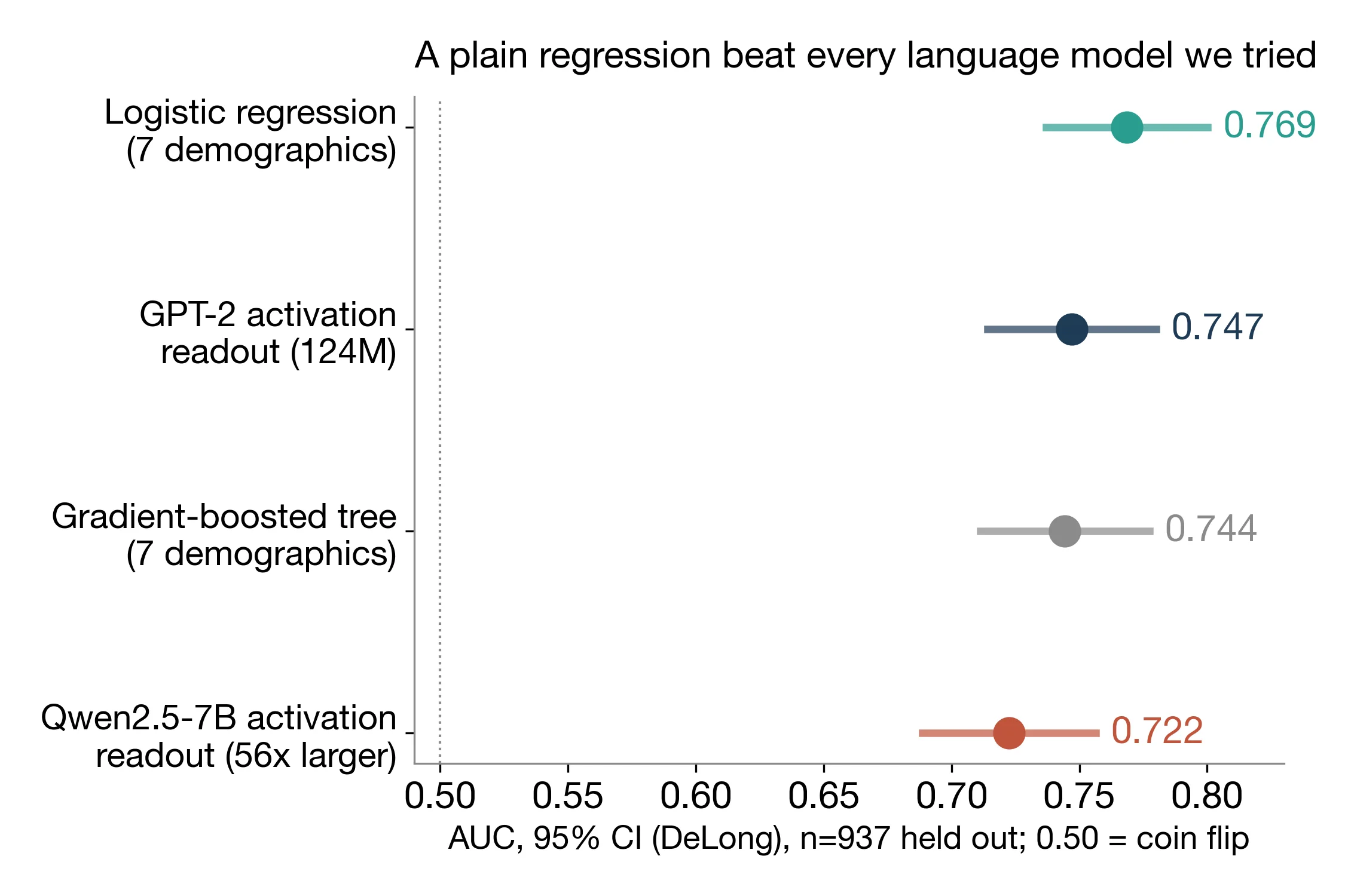
Model	AUC	95% CI
GPT-2 activation readout	0.747	[0.714, 0.780]
Gradient-boosted tree	0.744	[0.711, 0.777]
Logistic regression	0.769	[0.737, 0.800]

The intervals overlap, so the paired tests carry the weight here. We use DeLong’s test, a standard paired test for comparing two AUCs computed on the same respondents. The tree versus the readout is a statistical tie: the difference is -0.003 with a DeLong interval of [-0.018, +0.013] and p = 0.73. The logistic regression versus the readout is a different story: the regression is ahead by +0.022 AUC, with a DeLong interval of [+0.007, +0.036], a bootstrap interval of [+0.008, +0.036], and p = 0.003. The two interval methods agree. As flagged at the outset, the regression entered as an analysis-time baseline, so this is a result against a default comparator rather than a confirmed advance prediction; the DeLong test stands on its own terms either way.

What does +0.022 AUC mean in practice? AUC is the probability that a randomly chosen distressed respondent gets ranked above a randomly chosen non-distressed one. A gain of +0.022 means the regression correctly orders about two more pairs per hundred such comparisons than the language-model pipeline does. Where predicted risk decides who gets outreach first, that is a small but genuine improvement, and it comes from the cheaper, simpler, more interpretable model.

The twist: steering moves the model and changes nothing useful

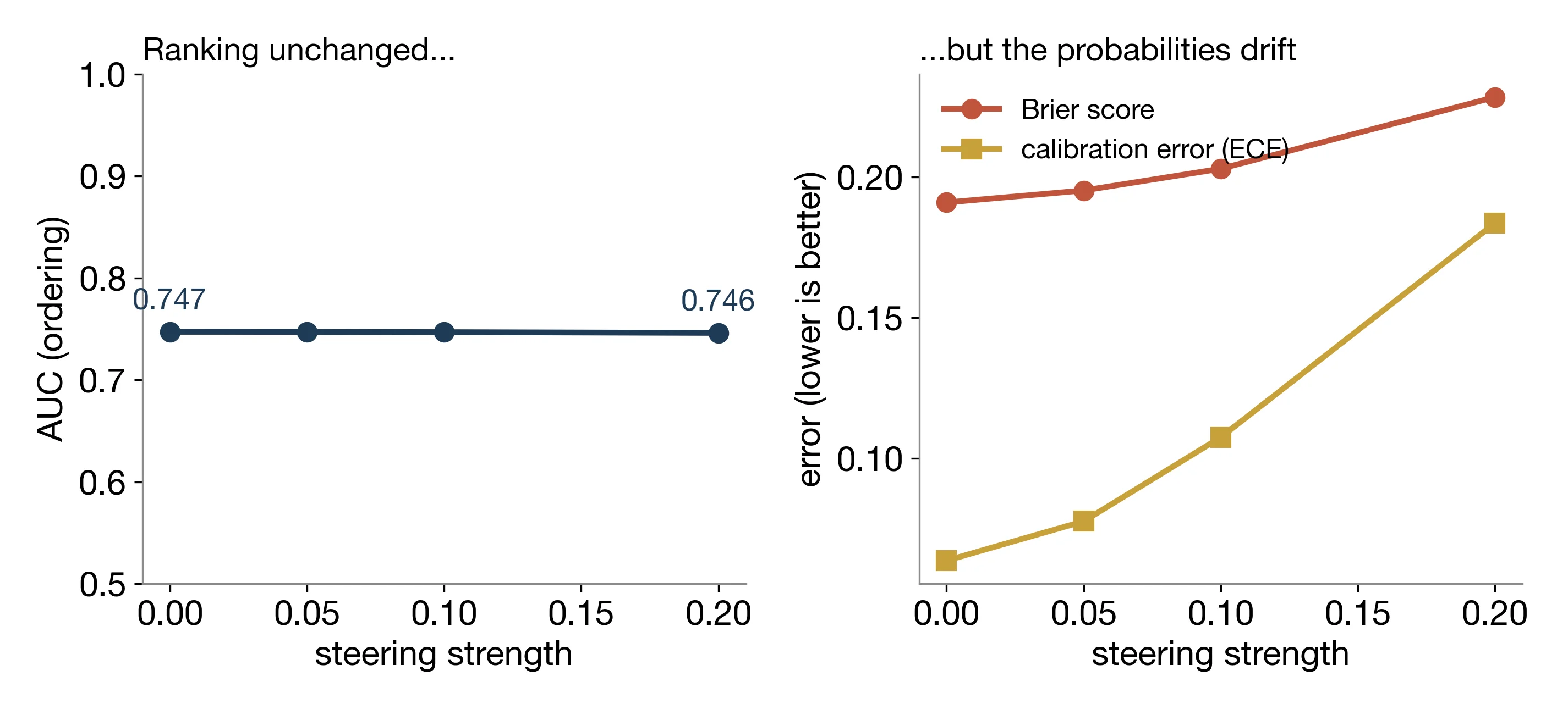
One natural objection: maybe the readout underuses the model, and a nudge to the internals would surface more signal. Activation steering does exactly that. We learn a distress direction in the model’s activation space: the difference in mean activations between distressed and non-distressed respondents in the build split, scaled to unit length. This is the same difference-in-means recipe part 2 dissects. Steering then adds K times the typical activation length times that unit vector to each evaluation respondent’s activations, and we re-score.

The three strengths we test are K = 0.05, 0.1, and 0.2, meaning the steering vector shifts the activations by 5, 10, and 20 percent of the typical activation norm. The AUC at those three strengths: 0.747, 0.747, 0.746. The ordering moves by at most one in the third decimal place.

The lazy reading of this null says the steering never reached the model. It did. At the strengths tested, the activations move by 5 to 20 percent of their own length, and the predicted probabilities shift by 4 to 16 percentage points on average, with a maximum shift of 0.35. The intervention lands. The shift is just nearly uniform across respondents, so everyone’s probability drifts together and almost nobody changes rank. AUC is a rank-based metric, and a rank-based metric cannot see a tide that lifts all boats equally.

Calibration degrades while the ordering stands still: the Brier score, a mean squared error for probabilities, rises from 0.191 to 0.228 at the strongest setting, roughly a 19% increase in probability error. The expected calibration error, the typical gap between a stated probability and the frequency actually observed at that probability, grows from 0.064 to 0.184: the average gap between what the model claims and what happens roughly triples, from about 6 percentage points to about 18.

This is close to the worst available trade. The ranking, the one thing steering set out to improve, stays where it started. The probabilities, which feed thresholds, caseload projections, and resource budgets, become less trustworthy at every step. If an outreach cutoff sits at “predicted risk above 50%,” a steered model that inflates everyone’s probability redefines who crosses that line without sorting anyone any better.

Why this result makes sense

We should have seen the steering result coming, and we did: the steering null is the prediction we wrote down in advance. The tabular side of the ledger is mixed: our advance document predicted the gradient-boosted tree would outpredict the language-model pipeline on AUC, and the observed result is a tie (-0.003, p = 0.73). The language model only ever saw the seven facts we put in the persona sentence. It cannot manufacture information that was never in its input; the best it can do is re-encode those seven facts, and any re-encoding through a 124-million-parameter text model is lossy. A logistic regression that uses the seven facts directly faces no such bottleneck.

The pipeline takes seven clean columns, smears them through a text encoder, and hands back roughly the same information with noise attached. The tree matching the readout and the regression coming out ahead are both consistent with that information argument, read after the fact; the argument caps what the model can know at the seven input facts without saying in advance whether the tree would tie or pull ahead.

The stopping rule we tripped and overrode

One pre-declared item remains, the most credibility-sensitive entry in the record. Before running anything, we worried that the personas might all look alike to the model: seven categorical facts produce sentences with near-identical wording, and if the activations failed to distinguish one persona from another, every respondent would get nearly the same vector, the readout would have nothing respondent-specific to learn from, and the test would be uninformative. The advance document therefore set a gate on cosine similarity, the cosine of the angle between two vectors, where 1 means the two point in the same direction. The rule: compute the mean pairwise cosine across personas, and if it exceeds 0.95, stop and report that the personas are too alike for the test to be informative.

The gate tripped. The raw-activation mean pairwise cosine came out at 0.998 against the 0.95 threshold, and the repository’s results file records the trip. We proceeded anyway, on a rationale adopted at analysis time. Raw transformer activations share one dominant common direction: every respondent’s vector contains the same large shared component, and when two vectors share a large common component, the angle between them is small no matter what else differs. Every pairwise cosine sits near 1, so the raw cosine measures the shared component and says little about whether respondents differ. After subtracting that shared mean component, distinct personas separate: the mean absolute cosine drops to about 0.35 over 200 personas, and the activation variance spreads over roughly 16 to 20 directions. That count is the effective subspace, a measure of how many directions carry the activation variance; computed two ways, it comes to 16.4 for mean-pooled activations and 19.9 for last-token activations. The readout’s 0.747 AUC is the operational proof, since a truly degenerate representation, one vector for everyone, would score 0.5. The override is an analysis-time judgment, we disclose it as such, and the centered diagnostics sit in results.json, the results file of the series’ replication repository that accompanies these articles.

Does the demographic signal depend on the case-enriched sample?

The case-enriched subsample raises a fair question: do the seven facts still predict distress in the population frame, where prevalence is about 14% rather than 0.36? The full complete-case frame holds 6,045 respondents. We refit the logistic regression on that frame with the survey’s design weights, using 5-fold cross-validation so that each respondent is scored by a model that never saw them. The weighted AUC comes to 0.759. The interval comes from a jackknife over replicate weights: HINTS ships 50 alternative weight columns, and recomputing the AUC under each one and pooling the spread yields a design-respecting standard error, giving [0.729, 0.790]. The unweighted AUC on the same frame, under the same cross-validation, is 0.767. A gap of less than 0.01 AUC suggests the demographic signal is stable to weighting; the regression’s performance does not look like an artifact of how we enriched the sample.

Scope, limits, and the question we closed

These numbers carry two standing limits and one limit we managed to close. First, the case-enriched subsample makes them method-comparison numbers, useful for ranking models against each other on a common footing; they are not population estimates of how well anyone can predict distress in the United States. Second, the language model knew only what we told it. Seven demographic facts in a persona sentence are a narrow channel, and a pipeline fed richer text, open-ended survey responses or clinical notes, would be answering a different question.

The third limit was model scale, and it is the one we closed before publishing. Everything above was first established for GPT-2 at 124 million parameters, and a fair objection was that a larger model might encode the persona less lossily. By the time we planned the larger run, the logistic regression’s 0.769 was the standing benchmark recorded in the repository, and the run was specified against it before it executed. We ran the same pipeline, identical subsample, split, readout recipe, and seed, on Qwen2.5-7B-Instruct, a model with 56 times GPT-2’s parameter count, reading activations at layer 14, on a free Colab T4 GPU. The larger model’s readout comes in at AUC 0.722 [0.689, 0.756] on the same 937 evaluation respondents: no better than GPT-2’s 0.747 (the intervals overlap) and below the logistic regression’s 0.769. A mid-size run with Qwen2.5-1.5B-Instruct, executed locally on a smaller balanced subsample (1,200 respondents per class, 817 evaluation respondents) to keep the job feasible on a laptop, lands at AUC 0.741 with a bootstrap interval of [0.705, 0.776], telling the same story. That is what the information argument predicted: scale cannot conjure signal the persona never contained. The zero-edit reproduction script, run_large_model.py, sits in the repository for readers who want to rerun it or swap in a different model; no language-model readout we tested reached the 0.769 benchmark.

Spend on the statistics

Across the three parts of this series, the classical statistics did the work every time. Part 1 built a do-no-harm guarantee, a regression adjustment that lets AI predictions sharpen a survey estimate without ever making the estimate worse, out of a linear adjustment and a variance formula. Part 2 asked whether a steering vector is secretly a regression gradient, and there the difference between a publishable steering effect and noise came down to seed counts and paired confidence intervals. Here in part 3, a logistic regression on seven facts outpredicts a language model reading those same facts (+0.022 AUC, p = 0.003), the steering null is diagnosed by separating rank metrics from calibration metrics, and the DeLong test is what lets us say any of it with confidence. The conclusion now extends to a model fifty-six times larger: the 7-billion-parameter run came in at 0.722, below both the small model and the regression. The burden of proof sits with any pipeline that proposes a language model where a regression already works, since the simple baseline is on the table at near-zero cost. We would spend on the statistics before we spend on the label. And for anyone who wants to re-test that conclusion, at this scale or another, the script is ready to run.