How to tell whether a double machine learning estimate is right

Before we report a causal effect that runs a machine-learning model inside the estimator, we can plant a known effect in simulated data and check whether the code recovers it. The check is the same planted-truth routine we use for any reimplementation:¹ specify a data-generating process we control, fix the true value of the parameter, and require the implementation to return it. What is new here is the estimator, and one way of building it that runs without error and returns the wrong number.

The wrong number is attenuated. On a design with a planted treatment effect of 1.0, a naive plug-in that regresses the outcome on a machine-learning prediction of the controls returns about 0.55, a little more than half the truth.² The code imports, runs, and hands back a coefficient in a reasonable range. A funder weighing a program whose benefit per unit of treatment has to clear 1.0 to pass a cost-benefit test would read 0.55 and defund a program that, in truth, pays for itself.

What double machine learning is

The setting is the partially linear model. We want the causal effect of a treatment D on an outcome Y, holding a set of controls X fixed:

Y = θ·D + g(X) + ε, and D = m(X) + ν.

Here θ is the one number we care about. The two functions g(X) and m(X) are nuisances: they describe how the controls shape the outcome and the treatment, and they can be high-dimensional and nonlinear. Double machine learning (DML), due to Chernozhukov and coauthors, lets a flexible machine-learning model estimate those nuisances while still recovering θ at the usual parametric rate with valid standard errors.³ The method exists because the obvious shortcut fails: dropping a regularized ML fit of g(X) straight into an outcome regression lets the model's bias leak into θ.

Two ingredients keep θ honest. The first is orthogonalization: residualize both Y and D on X and regress one residual on the other, so a small error in the nuisance estimate does not move θ to first order. This is the partialling-out logic of Robinson's semiparametric regression.⁴ The second is cross-fitting: estimate the nuisances on one fold of the data and form the residuals on a held-out fold, so the model's overfitting does not correlate with the residual used to estimate the effect. The naive plug-in skips both. It fits g(X) in-sample and never residualizes D, so the regularized fit absorbs treatment-linked variation in X and attenuates θ toward zero.

Check it against a planted effect

The tool is the same generic helper the companion piece builds:¹ verify_estimator plants a known effect, runs the estimator across many simulated draws, and reports whether the mean recovers the truth. We lift it in unchanged and point it at the two ways of estimating θ. The data-generating process confounds D through the same high-dimensional X that drives Y, so the nuisances are real work, and the planted effect is 1.0.

Planting the effect is concrete: we choose the number, here 1.0, and set it as θ, the coefficient on D in the line that generates Y (Y = θ·D + g(X) + ε above). The estimator never sees that number; a correct one has to recover it from the simulated data alone. In the code below, that number is the third argument to verify_estimator.

from verify_estimator import verify_estimator, report
from dml_plm import simulate, naive_plugin, dml_plm

# plant a known effect of 1.0; confounding runs through 20-dim X
report("naive ML plug-in",      verify_estimator(naive_plugin, simulate, 1.0, tol=0.10, reps=50), 1.0)
report("double ML (cross-fit)", verify_estimator(dml_plm,      simulate, 1.0, tol=0.10, reps=50), 1.0)

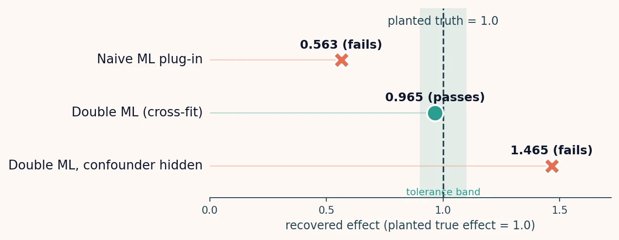
# naive ML plug-in       planted 1.00 | recovered 0.563 +/- 0.003 (MC SE) | bias -0.437 | FAIL
# double ML (cross-fit)  planted 1.00 | recovered 0.965 +/- 0.005 (MC SE) | bias -0.035 | PASS

The naive plug-in and cross-fitted DML part ways against the same planted truth. On a single reference draw the split is already visible: the naive plug-in returns 0.55 while DML returns 0.97, with a nominal 95% confidence interval of [0.90, 1.03] that covers the planted 1.0.² Averaged over many draws, so a single unlucky sample cannot be mistaken for the pattern, the naive plug-in's attenuation is systematic, not sampling noise.

Estimator (planted effect = 1.0)	Recovered (50-draw mean)	What the check showed
Naive ML plug-in (in-sample, no orthogonalization)	0.56	attenuated toward zero; fails the check
Double ML (cross-fitted, orthogonal)	0.97	recovers close to the planted effect; passes

A run of it looks exactly like a run of the correct estimator, which is the whole reason to plant a truth and check recovery rather than eyeball whether the coefficient looks reasonable.

Where the check stops

The check earns two limits, and stating them plainly is part of using it.

The first is that passing is not exact recovery. DML returns about 0.97, not 1.0. That residual is finite-sample noise from estimating the nuisances on a data set of this size, and it shrinks as the sample grows; the confidence interval covers the truth, so the gap is not evidence of a bug. Reading 0.97 as "the effect is 1.0 recovered exactly" overstates what the check delivers. It says the estimator is close and consistent on this process, not that it is perfect on any one draw.

The second limit is the one that matters for a policy number. The check confirms that DML recovers a planted effect given the controls we simulate. It says nothing about whether the controls we use on the real data contain every confounder. Suppose a variable U moves both the treatment and the outcome and never enters X. Run DML on that world, with U omitted from the controls, and the estimate is biased for the true effect: a mean of about 1.46 against a planted 1.0.² When we build the simulation, we choose what goes into X, and we naturally build the same control set we plan to use, so our simulated X omits U exactly as our real analysis does. The simulation never generates the confounding, the check reports clean recovery, and the omitted confounder passes unseen. DML removes regularization bias from the nuisances; it does not manufacture the identifying assumption that X is complete. That assumption still has to be defended on its own, from how the treatment was assigned.

The reproduction

The generic verify_estimator helper, the DML and naive estimators under test, and the worked check that produced the numbers above are at github.com/dphdame/tooearlytosay-analysis. Clone it, plant an effect, and the check reports whether each estimator recovers it; the naive plug-in asserts to FAIL and the run exits nonzero.

The orthogonal moment, in more detail

DML estimates θ from a moment condition built on the two residuals, Y - E[Y|X] and D - E[D|X]. That moment is Neyman-orthogonal: its derivative with respect to the nuisance functions is zero at the truth, so a first-order error in the machine-learning estimates of E[Y|X] and E[D|X] does not propagate into θ. The naive plug-in uses a moment that is not orthogonal, so its nuisance error enters θ directly.

Orthogonality removes the first-order bias but not a second source: the overfitting correlation between the nuisance fit and the residual it is subtracted from. Cross-fitting removes that by estimating each observation's nuisance value on a fold that excludes it, so the fitted value and the residual are independent. Together the two give θ its parametric rate and a standard error we can trust. The formal statement, including the regularity conditions on the nuisance estimators, is in Chernozhukov and coauthors.³ The planted-truth check is the applied shadow of that theory: it confirms recovery on a process we control, which is necessary for trust and, as the omitted-confounder case shows, not sufficient for it.

Closing

Folding a machine-learning model into an estimator does not change what verification asks. The question is whether the implementation recovers the effect we planted and whether the design identifies the effect we claim, not whether the code ran. Double machine learning answers the first when the naive plug-in does not; neither answers the second, which is ours to defend. The routine travels to any estimator we can simulate under a known truth, in code written by us, by a colleague, or by an assistant.

Notes

1. Cholette, V. (2026, June 17). How do we know an AI's estimator does what we meant? Too Early To Say. https://tooearlytosay.com/research/methodology/validate-ai-econometric-code/ The verify_estimator helper and the planted-truth routine are built there; this piece reuses them unchanged.
2. Numbers are from seeded, rerunnable reproduction code (github.com/dphdame/tooearlytosay-analysis, validate-double-ml). Against a planted true effect of 1.0 on the reference seed, the naive ML plug-in recovers 0.554 (bias -0.446) and cross-fitted double ML recovers 0.968 with a nominal 95% confidence interval of [0.904, 1.032]. Averaged over 50 independent draws the naive plug-in recovers a mean of 0.563 (Monte Carlo SE 0.003) and double ML a mean of 0.965 (Monte Carlo SE 0.005). On a data-generating process with a confounder omitted from the controls, double ML recovers a mean of 1.465 (bias +0.465) against the planted 1.0.
3. Chernozhukov, V., Chetverikov, D., Demirer, M., Duflo, E., Hansen, C., Newey, W., & Robins, J. (2018). Double/debiased machine learning for treatment and structural parameters. The Econometrics Journal, 21(1), C1–C68. https://doi.org/10.1111/ectj.12097
4. Robinson, P. M. (1988). Root-N-consistent semiparametric regression. Econometrica, 56(4), 931–954. https://doi.org/10.2307/1912705