Matching in Python: a balanced covariate table doesn't make the estimate valid

Before we trust a matched estimate, we should check that a comparison actually existed for every treated unit, not just that the balance table looks clean. Matching pairs each treated unit with a control that has a similar propensity score, then reports the standardized mean difference (SMD) on each covariate as evidence the two groups are comparable. When every SMD lands under the usual 0.10 rule, the table reads as success. The table can read as success while a share of the treated units had no comparable control at all, and there the estimate is built on comparisons that were never really there.

To see the gap, we plant a known effect and ask matching to recover it. Two covariates drive who gets treated; the same covariates drive the outcome, so this is selection on observables and matching should work. We build one wrinkle in: treatment is concentrated enough in the tail of the first covariate that the most-treated units have almost no controls near them. The planted effect of the treatment on the outcome is 2.0, the same for every unit.

The clean table and the wrong number

Nearest-neighbor matching on the propensity score is a few lines. For each treated unit we find the control with the closest score and difference the outcomes; the average is the estimated effect on the treated.

import numpy as np

# ps: estimated propensity, d: treated (1/0), y: outcome
def nn_match_att(ps, d, y, keep=None):
    d = d.astype(bool)
    treated = np.where(d if keep is None else (d & keep))[0]
    control = np.where(~d)[0]
    ps_c = ps[control]
    matched = [control[np.argmin(np.abs(ps_c - ps[i]))] for i in treated]
    return np.mean(y[treated] - y[matched])

print(round(nn_match_att(ps, d, y), 2))   # -> 2.21 on the reference draw (planted 2.0)
# max |SMD| after matching: 0.08 -> "balanced" by the 0.10 rule

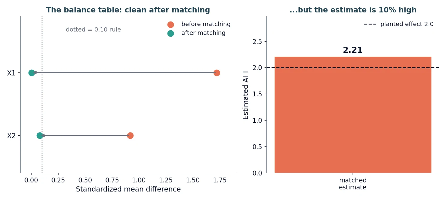
When we match, we get 2.21 against the planted 2.0, about 10% high, and the balance table gives no indication anything is wrong. Before matching the groups were far apart, with an SMD of 1.72 on the first covariate and 0.92 on the second; after matching the largest SMD is 0.08, under the 0.10 rule. By the standard evidence the match succeeded, yet we are still 10% off.

The bias is not a fluke of one dataset. When we run 200 simulated samples, the matched estimate averages 2.23 and lands above the true 2.0 in 84% of them, with a standard deviation of 0.22, so this is a direction, not sampling noise around the right answer. And the balance table is a weak alarm: across those same 200 samples we see a median largest SMD of 0.102 after matching, clearing the 0.10 rule only 48.5% of the time. About half the time a practitioner sees a passing table, and even then the estimate runs high. The balance check and the bias are close to independent.

The check that reveals it: common support

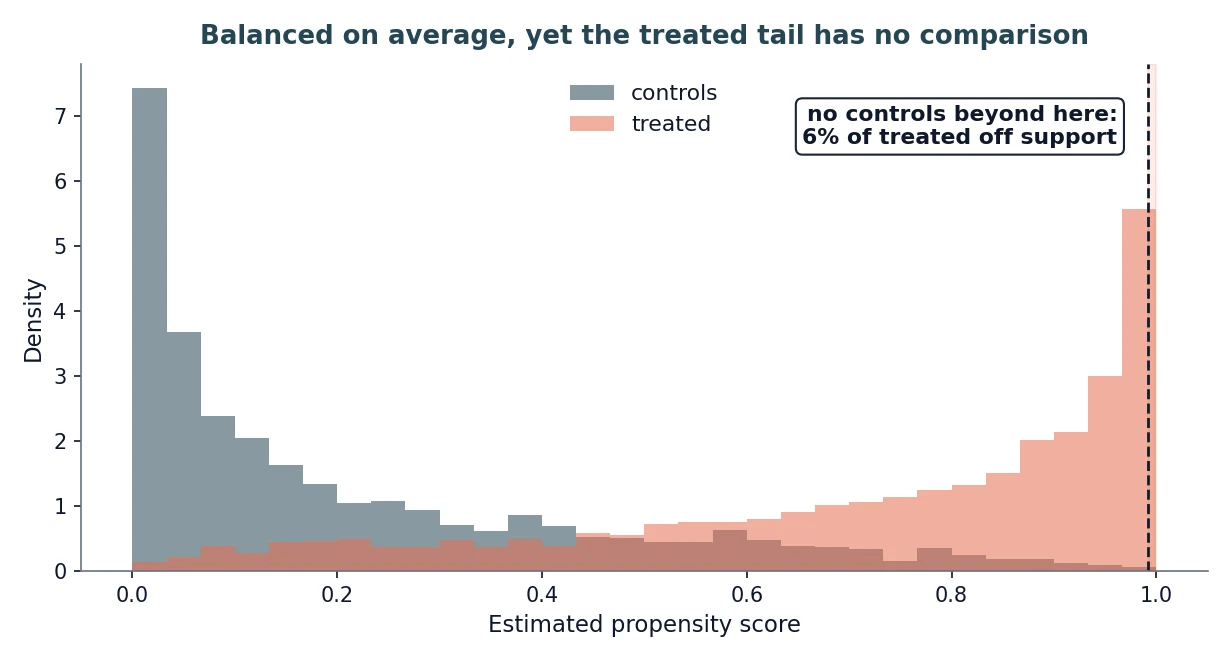
The number that would have shown this is the share of treated units with no comparable control. A treated unit whose propensity is higher than every control's has nothing to match to, so nearest-neighbor pairs it with a distant control, and because the outcome rises steeply in that tail the mismatch enters as bias. One line reports the share.

def off_support_share(ps, d):
    """Fraction of treated units with a propensity above every control's."""
    d = d.astype(bool)
    return np.mean(ps[d] > ps[~d].max())

print(round(off_support_share(ps, d) * 100, 1))   # -> 6.0% of treated off common support

On the reference draw 6% of treated units sit off common support (a mean of 8.9% across the 200 samples). The balance table cannot report this, because an average difference over the matched pairs does not register whether the match was close or distant. The fix is to estimate the effect only where a comparison exists. Trimming units with an estimated propensity outside [0.1, 0.9] — the rule of thumb from Crump, Hotz, Imbens & Mitnik (2009), not their variance-minimizing cutoff — drops the off-support tail and re-matches.

keep = (ps >= 0.1) & (ps <= 0.9)              # Crump et al. (2009) trimming
print(round(nn_match_att(ps, d, y, keep), 2))  # -> 2.04, keeping 62% of treated

# the planted-truth check: a valid estimate recovers 2.0 within tolerance
assert abs(nn_match_att(ps, d, y, keep) - 2.0) < 0.1   # trimmed: passes
assert abs(nn_match_att(ps, d, y) - 2.0)       < 0.1   # naive: FAILS, raises AssertionError

When we trim, we get 2.04, keeping 62% of the treated units, and the balance table is still clean. Recovering 2.04 rather than exactly 2.0 is sampling noise on this one draw, not leftover bias: across the 200 samples the trimmed estimate averages 2.00. The fix is robust across two standard routes. With the [0.1, 0.9] trim we get 2.04; with the field-standard caliper of Austin (2011), which matches on the logit of the propensity and drops the 3.7% of pairs with no close comparison, we get 2.05. Two different, citable ways of restoring common support land in the same place.

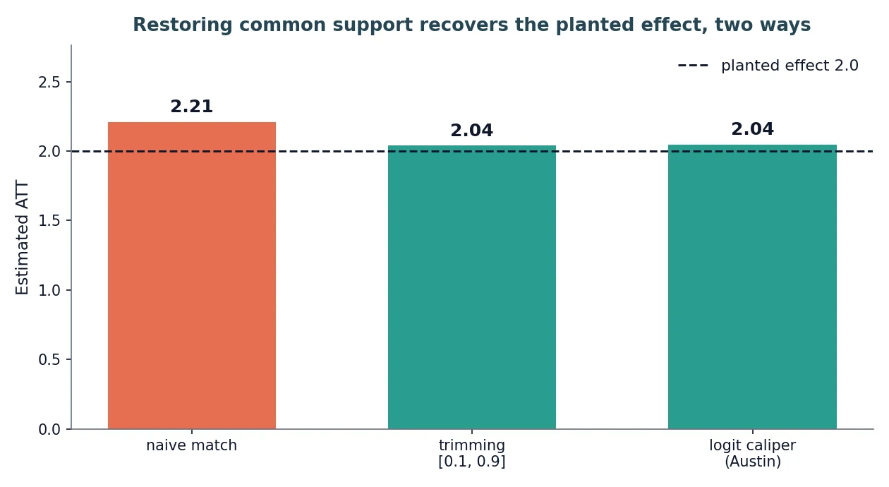
One caution comes out of the same setup. A caliper on the raw propensity, the more common default, does not help here: at widths from 0.20 down to 0.01 we still get 2.21 and drop 0% of units, because the propensity scale compresses near 1: the off-support treated sit a tiny raw distance from the nearest available controls, which are themselves sparse up there. The same caliper on the logit scale, where the tail is stretched out, drops them and recovers the effect. Match and set calipers on the logit of the propensity.

The limit no balance table can defend: unconfoundedness

Common support is a testable property, and the diagnostic above reveals its failure. The deeper assumption is not testable. Matching identifies the effect only if treatment is as good as random given the covariates we condition on — unconfoundedness, the claim that no unobserved factor moves both treatment and outcome. To see what that costs, we add exactly such a factor, then run the whole honest workflow anyway: estimate the propensity on the observed covariates, trim to common support, match, and check balance.

Every observable check passes: we get balanced covariates, with a largest SMD of 0.065, and restored overlap. We get 3.23 against the true 2.0, about 60% too high, and nothing computable from the observed data indicates it. This is the limit of the diagnostic: an overlap check cannot detect a confounder that is not in the data. The unobserved factor never appears in the propensity model, the balance table, or the overlap diagnostic, because we cannot condition on what we did not measure.

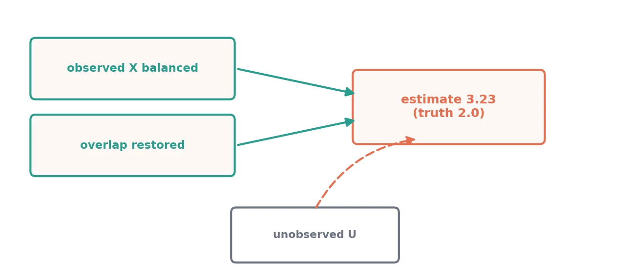
This is the same untestable assumption that double machine learning also rests on; the difference is where each method spends its effort. Double machine learning is about orthogonalization, removing the bias that comes from estimating many nuisance parameters. Matching is about overlap, whether a comparable control existed at all. Both stop at conditional independence, which is an argument about the world rather than a quantity in the data.

What to check, before the estimate

Three checks matter more than the balance table, in order.

1. Report an overlap diagnostic, not just a balance table. The share of treated units off common support is the number that would have shown the 2.21 problem. A clean SMD table is necessary, and on its own it is not sufficient.
2. Match and set calipers on the logit of the propensity. On the raw scale the non-overlap that biases the estimate does not show up as distance, because propensities compress in the tails; the logit scale keeps it visible.
3. State the unconfoundedness assumption in words a referee can attack. Name the unobservable that could move both treatment and outcome, and the estimand trimming leaves you with, because no balance table or overlap plot provides evidence for either one.

The matched number is the output, read alongside the overlap that supports it and the argument for unconfoundedness that no statistic can settle. The judgment the reader owes is whether a comparison existed and whether the design identifies the effect, not whether the covariates balanced.

Reproduction

The full simulation, including the selection-on-observables data generation, nearest-neighbor matching, the balance table, the common-support diagnostic, the [0.1, 0.9] trimming and logit caliper, and the unobserved-confounder case, is at github.com/dphdame/tooearlytosay-analysis. The setup uses simulated data with a fixed seed, so results reproduce exactly, and the figure generator asserts its own layout and exits nonzero on a collision.

References

- Crump, R. K., Hotz, V. J., Imbens, G. W., & Mitnik, O. A. (2009). Dealing with limited overlap in estimation of average treatment effects. Biometrika, 96(1), 187-199.
- Austin, P. C. (2009). Balance diagnostics for comparing the distribution of baseline covariates between treatment groups in propensity-score matched samples. Statistics in Medicine, 28(25), 3083-3107.
- Austin, P. C. (2011). Optimal caliper widths for propensity-score matching when estimating differences in means and differences in proportions in observational studies. Pharmaceutical Statistics, 10(2), 150-161.