Regression discontinuity in Python: getting the effect at the cutoff right

RDD reads a treatment effect off a seam. Units just above a cutoff are treated; units just below are not; the jump in the outcome at that cutoff is the effect. In Python, estimating that jump takes only a few lines of regression code. That ease creates a risk: treating the printed coefficient as the finding. It is the most fragile part of the analysis.

To see why, we can plant a known effect in simulated data and ask different estimators to recover it. The true jump at the cutoff is set to 0.75. The outcome varies smoothly with the running variable in a way that is not exactly polynomial, and the treatment effect increases away from the cutoff. That last feature matters: the effect at the cutoff (0.75) is not the same as the average effect among the treated (about 1.5). RDD is designed to recover the local effect at the cutoff, not the average effect elsewhere.

The exercise turns on two questions an analyst should answer before reporting any RDD estimate, both of which matter more than which estimator produced the number: would the result survive a reasonable change in modeling choice, and does the cutoff isolate the treatment at all.

Problem 1: Functional form drives the estimate

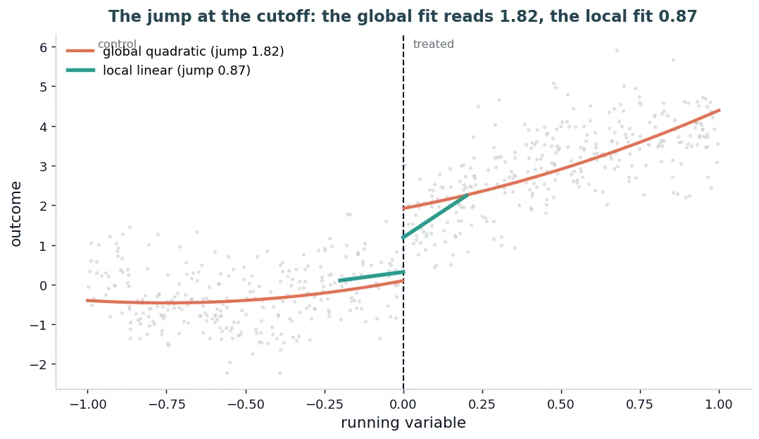
Start with the common approach: we regress the outcome on the running variable, its square, and a treatment indicator across the full sample, and read the treatment coefficient as the effect. We get 1.82, against a true value of 0.75.

import numpy as np, statsmodels.api as sm

rng = np.random.default_rng(20260704)
X = rng.uniform(-1, 1, 2000)              # running variable
D = (X >= 0).astype(float)                # treated above the cutoff
Y = np.sin(3*X) + 0.5*np.exp(X) \
    + (0.75 + 1.5*X)*D + rng.normal(0, 0.7, 2000)   # true jump at cutoff = 0.75

cols = sm.add_constant(np.column_stack([D, X, X**2]))
print(sm.OLS(Y, cols).fit().params[1])    # -> 1.82, not 0.75

The regression is coded correctly. The trouble is that a single global polynomial is doing too much. It has to fit both the smooth curvature in the outcome and the discontinuous jump at the cutoff, and it cannot do both cleanly, so part of the curve gets charged to the treatment.

A natural response is to increase the polynomial order. Increasing the order only exposes the problem: different, equally defensible specifications produce different answers, and all three run without warning.

Global polynomial order	Effect at the cutoff (true value 0.75)
Quadratic	1.82
Cubic	0.81
Fifth-order	0.74

All three models are defensible, and the data alone cannot single out which to trust. Nothing in the regression output says which order is right, and the estimate reported is whichever one the analyst happened to pick. Global polynomials are a reasonable tool in general. The problem here is that a global fit forces a functional-form decision the data cannot confirm, and the treatment effect inherits that arbitrariness.

The fix: estimate locally

A local approach avoids guessing the global shape. Instead of fitting one curve to the entire sample, we fit simple models on each side of the cutoff using only nearby observations, and weight points closer to the cutoff more heavily. The reason is that any smooth function is approximately linear in a small neighborhood, so a local linear fit works without committing to a global polynomial.

def local_linear(X, D, Y, h):
    m = np.abs(X) <= h                    # keep points within bandwidth h of the cutoff
    w = 1 - np.abs(X[m]) / h              # triangular weights, heavier near the cutoff
    Z = sm.add_constant(np.column_stack([D[m], X[m], D[m]*X[m]]))
    return sm.WLS(Y[m], Z, weights=w).fit(cov_type="HC3")

fit = local_linear(X, D, Y, h=0.20)
print(fit.params[1])                      # -> 0.87 on this draw

On a representative draw we get 0.87, with a 95% confidence interval that covers the true value of 0.75. Averaged across many simulations, the estimate centers on the truth. More important than any single number is the pattern: across different underlying outcome shapes, the local estimator stays stable while global polynomials swing with curvature. That stability is the point.

What still requires judgment

Local estimation does not eliminate all choices. First, the bandwidth matters. A narrow window uses observations very close to the cutoff and targets the local effect, but with higher variance. A wider window increases precision but pulls in observations where the treatment effect is larger, shifting the estimate upward toward the treated average of 1.5. As the bandwidth approaches the full sample, the local estimator becomes global again.

Second, recovery is approximate, not exact. Even in clean simulations, estimates vary across samples and bandwidths, and that variation is part of the result, not a nuisance to ignore. In practice, bandwidth selection should follow established data-driven methods, and results should be reported with sensitivity to reasonable alternatives.

Problem 2: The cutoff may not isolate treatment

Even a well-executed local design can answer the wrong question. RDD identifies a treatment effect only if crossing the cutoff changes one thing: the treatment of interest. If multiple programs or policies activate at the same threshold, the observed jump combines all of them.

Consider a concrete case: an income cutoff that determines eligibility for both a health program and a housing subsidy. An RDD at that threshold estimates the combined effect of both interventions, and no choice of bandwidth or functional form can separate them within the design. Standard diagnostics may not help. A density test can confirm that units are not sorting around the cutoff, but it cannot catch that several treatments change at the same point, a limit no diagnostic inside the design can detect, because none is built to. When we add a second program at the same threshold, we get about 1.18 from the local fit against a true effect of 0.75, and the density test still passes cleanly. The design works mechanically and still delivers the wrong estimand.

This is the more serious threat. Functional-form issues bias the estimate; identification failures redefine it.

What to prioritize, before the estimate

Three checks matter more than the coefficient itself, in order.

1. Does the cutoff isolate the treatment? If several interventions change at the threshold, the estimate bundles them. This has to be argued from institutional knowledge, not inferred from the data alone. Clarify whether the design is sharp or fuzzy, and what estimand follows.
2. Is the estimate robust to defensible choices? Vary bandwidths, functional forms, and specifications. If the estimate moves across them, report the range. Stability is evidence; a single preferred number is not.
3. What exactly is being estimated? RDD recovers a local effect at the cutoff. When treatment effects vary with the running variable, that differs from the average effect among participants.

The value the code returns is the output, read alongside its uncertainty and its identification argument; the finding is whether the design and the estimate hold up.

Reproduction

The full simulation framework, including the data generation, the global and local estimators, the bandwidth variation, and the compound-treatment case, is at github.com/dphdame/tooearlytosay-analysis. The setup uses simulated data with a fixed seed, so results reproduce exactly. Modifying the outcome shape or the treatment effect tests how each estimator behaves under alternative conditions.