Difference-in-differences (DiD) is the workhorse of policy evaluation. One place changes a policy, similar places do not, and we compare how some outcome moves in the treated place against how it moves in the others. The untreated places stand in for what would have happened to the treated place without the policy. When their trends would have stayed parallel, the comparison gives us a clean read on what the policy did.
Real policy settings strain that logic in two ways at once. The places adopt at different times, so there is no single clean before-and-after. And there are very few of them: often one treated state and a handful of comparison states. With only a handful, the two checks we lean on to defend a DiD each fail in a specific way. The first, a test that the groups were moving together before the policy, has little power when the panel is short, so it rarely catches a real violation. The second, the standard errors behind the confidence interval, come from large-sample approximations that assume many independent groups; with three or four, the formulas understate the true uncertainty and the interval comes out too narrow. The reported estimate looks more precise than the data can support.
A recent method takes direct aim at that corner. The rolling
difference-in-differences estimator of Lee and Wooldridge, packaged as
the Stata command lwdid, handles staggered adoption and
carries an explicit small-sample path, with inference designed for a
handful of units rather than a crowd.1
This piece is about how to put it to work: what it estimates, the
choices it asks of us, how to read what it returns, and how to check our
own answer on a real few-unit policy problem.
For readers who work in Python, or who want the logic in the open rather than inside a package, we rebuild the small-sample procedure from its description in a few hundred lines. The rebuild puts the method within reach of a non-Stata audience, and running it on data where we set the true effect ourselves shows how the method behaves, and which choices change the estimate, before we apply it to real data where we cannot check it. The estimator’s formal properties are established in the underlying papers, which also benchmark it against synthetic control and the standard staggered-DiD commands; our aim is practical, to show how to apply the method to a few-unit policy problem, in code we can read, and how to check the answer it gives.
Rolling difference-in-differences, in plain English
Start with what we are trying to estimate. For each group of units that adopts the policy at the same time, we want the average treatment effect on the treated (ATT): how that group’s outcome moved after adoption relative to units not yet treated, read group-by-group across time and then averaged into an event-time path. Like every DiD, it rests on one assumption: absent the policy, treated and comparison units would have moved in parallel.
We can look at each unit’s pre-treatment periods to describe what it was doing before the policy: its average level, or its level plus a linear trend, or its level, trend, and seasonal swing. We subtract that description from the unit’s later outcomes, and what remains is the part the past did not predict. Then, in each post-treatment period, we compare that remainder for treated units against not-yet-treated units with a simple cross-sectional regression. The coefficient is the treatment effect for that period.
Two features make this worth the trouble in small-sample policy work. The detrending choice lets each unit keep its own linear trend, which relaxes the strict parallel-trends requirement that sinks so many few-unit designs. And the same subtraction, applied to the pre-treatment periods, hands us placebo tests for free: if the method is sound, the estimated effect before the policy should sit near zero.
The method needs four columns: an identifier for each unit (here, each state), a time index (the quarter or the year), a marker for the period when each unit adopted the policy, with a zero for units that never did, and the outcome we care about. What it does require is enough pre-treatment periods, because we can only subtract a pattern we can estimate from the pre-period. A mean asks for almost nothing; a linear trend needs at least two pre-treatment periods; a quarterly seasonal pattern needs enough quarters to estimate its four seasonal terms.
Rebuilding it in Python
Before applying the method to a real policy question, it helps to run it where we already know the answer, and data for that comes in two kinds. We can simulate a panel ourselves: choose the number of treated and control units, plant a treatment effect we know, and build in the trend differences and seasonality we want to test. Or we can use a real policy panel with staggered timing and a small control pool. The difference between them is the answer key. Simulated data comes with the true effect we set, so we can score each estimate against it; real data does not, so it shows whether the method behaves on messy inputs but cannot tell us whether an estimate is correct. We start with the simulated panel for that reason, dialing the trend gap and the seasonal swing up and down to watch the estimator respond. Once the code reproduces effects we planted, running it on a real panel becomes a genuine test of whether the method holds where we cannot check the answer.
Running it where we know the answer teaches four things about applying the method, with the true effect set to 1.0.
First, when trends are genuinely parallel, the transformation choice barely matters. In the easy case (6 treated and 6 control units, parallel trends, no seasonality), all three transforms land near the truth: demean gives an ATT of 0.958 (standard error, SE, 0.089), detrend gives 0.859 (SE 0.136), and detrend-plus-seasonality gives 0.823 (SE 0.169). All three reject zero on every inference mode: exact-t and HC3 p-values fall well below 0.001, and randomization inference returns p around 0.002. Adding flexibility costs precision; the SE rises from 0.089 to 0.169 as we move from demean to detrendq. It barely moves the estimate, because the trends really are parallel.
Second, when trends diverge, the transformation choice decides the answer. In the hard case (3 treated and 3 control units, diverging treated-versus-control trends, quarterly seasonality), demean reports an ATT of 2.061, roughly twice the truth, because demeaning ignores the differential treated-unit trend. Detrend recovers the truth at 1.127. Detrend-plus-seasonality lands in between at 1.525, because three extra seasonal parameters estimated on an eight-period pre-window inflate variance and leave some trend uncorrected; with a longer pre-window the seasonal version closes that gap. The spread from 2.061 to 1.127 is the lesson in two numbers, and detrendq’s 1.525 is the reminder that more flexibility is not free when pre-treatment periods are scarce.
Third, the spread across the transformations is itself a diagnostic we can read. When the three agree, as in the easy case, the parallel-trends assumption is doing no harm. When they diverge, as in the hard case, the divergence tells us which assumption is load-bearing.
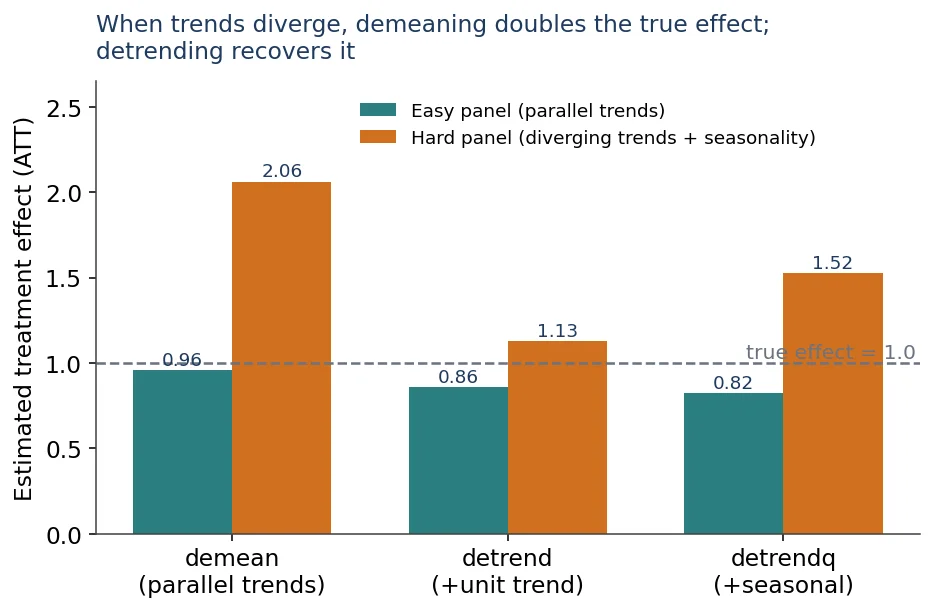
Easy panel: all three transforms land near the true effect of 1.0. Hard panel: demeaning doubles it, detrending recovers it, the seasonal variant falls in between.
Fourth, with few units, the inference mode decides how much we can claim. In the hard case, both estimates run on the same six units, so the exact-t uses four degrees of freedom (N minus two) either way; the contrast is about honesty, not sample size. Demean’s exact-t p-value is 0.001, false confidence built on a biased point estimate, while its randomization-inference (RI) p-value is 0.041. Detrend, the honest estimate, reports an exact-t p of 0.108 and an RI p of 0.179: six units cannot reject zero, and randomization inference says so plainly. The staggered run reinforces this. Under detrend, the pre-treatment placebo cells hug zero (event time r = -1: -0.014; r = -2: -0.001; r = -3: -0.020), validating the design, while post-treatment effects drift from about 1.0 up to about 2.0 at the latest event times. That upward drift is the method’s real fragility: extrapolating a trend estimated on a short pre-window far past that window injects error that grows with event time.
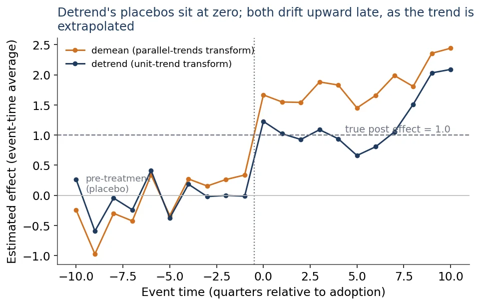
Detrend’s pre-treatment placebos sit at zero; both transforms drift upward at late event time as the estimated trend is extrapolated past its pre-window.
The table below lays out each part of the simulated analysis: how it is set, what it checks, and why that matters.
What each part of the analysis checks
| Part of the analysis | How we set it | What it checks | In plain terms |
|---|---|---|---|
| Panel structure | 6 treated + 6 control (easy); 3 treated + 3 control (hard); 16 quarterly periods | Whether the estimator behaves with realistically small unit counts | Real small-N policy studies have only a few places; this is the setting the method is meant for |
| Treatment timing | One common adoption period (easy and hard); staggered cohorts adopting at three different times (event study) | Single-period logic and the cohort-by-time-to-event aggregation | Some policies start everywhere at once, others phase in across years; we test both |
| Known effect | True effect set to 1.0 in every design | Grading: every estimate is scored against a fixed, known answer | We plant the answer so we can tell whether the code finds it |
| Diverging trends | Treated places trending faster than controls (hard and staggered); same trend (easy) | Whether the method recovers the truth when parallel trends fail; isolates the demeaning bias | Treated and comparison places can be on different paths even without the policy, the case that breaks plain DiD |
| Seasonality | A fixed quarter-of-year pattern switched on (hard) or off (easy and staggered) | Whether seasonal swings contaminate estimates the seasonal adjustment should remove | Outcomes that rise and fall by quarter can fool the estimate unless removed first |
| Transformations | demean, detrend, detrendq, each fit on pre-treatment periods only | Sensitivity: the spread across the three is the diagnostic (easy 0.96/0.86/0.82; hard 2.06/1.13/1.52) | The three ways to strip out a unit’s past; if they disagree, the answer depends on a modeling choice |
| Inference modes | exact-t, HC3-robust, and randomization inference (2,000 permutations) | Honesty at small N: hard-case demean exact-t p=0.001 vs randomization p=0.041; detrend randomization p=0.179 | Three ways to compute the margin of error; with few units, the honest ones admit how little we can prove |
| Pre-policy placebo periods | Effect estimated for periods before adoption, under detrend (about -0.01 to -0.02) | Design check: estimates near zero before the policy confirm the trend fit | The method should find nothing before the policy starts; near-zero here means it is not inventing effects |
| Easy vs hard contrast | The same estimator on a parallel-trends panel and on a diverging-trends-plus-seasonal panel | Where the method is stable (all transforms near 1.0) versus where it breaks (demean 2.06 vs detrend 1.13) | The same tool on an easy and a hard problem, to show where it can be trusted and where it cannot |
Arizona’s Medicaid freeze: small-N DiD in practice
The Arizona Medicaid enrollment freeze is the kind of setting small-sample DiD was built for. On July 8, 2011, Arizona froze new and re-enrollment in Medicaid for childless adults below 100% of the federal poverty level. The policy question is direct: when a state shuts a coverage door, who shows up at the hospital uninsured? The rolling-DiD paper measures two insurance-composition outcomes among adults aged 50 to 64 admitted with non-deferrable diagnoses, such as heart attacks and strokes: the share of hospital discharges whose primary payer is Medicaid, and the share recorded as self-pay.3 A rising self-pay share means more uninsured hospitalizations, which is consequential for both patients and the hospitals absorbing the cost.
The data come from the State Inpatient Databases (SID) within the Healthcare Cost and Utilization Project (HCUP), spanning the first quarter of 2008 through the fourth quarter of 2013. Arizona is the treated state. Arkansas, Maryland, and New Jersey serve as controls, none having contracted Medicaid comparably in the window. Discharge microdata are aggregated to the state-by-quarter level, yielding a balanced panel of four units, one treated and three control, with a common treatment date in the third quarter of 2011 and a quarterly frequency.
Four features make this hard, and each maps onto something the
lwdid implementation of the rolling estimator is built to
handle. First, four units is a small-sample problem. Cluster-robust
standard errors and large-sample asymptotics are unreliable when the
cluster count is three controls plus one treated state; this is why
exact-t, HC3, and randomization inference enter the picture rather than
conventional standard errors. Second, hospital discharge composition
carries quarter-of-year seasonality, which the deseasonalizing options
(demeanq, detrendq) are meant to strip out.
Third, a standard two-way fixed-effects (TWFE) DiD event study shows
differential pre-trends: Arizona’s Medicaid share was already rising
relative to controls before the freeze, reflecting an earlier
waiver-based expansion. That pre-existing drift biases the unadjusted
DiD toward zero, and the unit-specific detrending (detrend,
detrendq) is designed to remove exactly this kind of trend.
Fourth, the discharge records are repeated cross-sections, yet the
rolling logic still applies once outcomes are formed at the
state-quarter level.
The control pool stays thin for a real reason. Few states ran a comparable Medicaid contraction in the same window, so we cannot pad the comparison group with 40 more states that happen to resemble Arizona. The single common treatment date here is also a simplification of the broader policy world; many real Medicaid changes arrive staggered across states and years, which is the case the rolling estimator is more generally written to address.1 Arizona is the clean common-timing instance; the staggered version is where the method’s machinery is meant to scale.
Applying it to a few-unit panel: a checklist
Applying the method is not just running it once. With four units and adjustment options that each move the estimate, the answer we report depends on choices we make, so applying it well means running it several ways and seeing whether the answer holds. The checklist below is the minimum we would run on our own panel before reporting a result from it.
Pre-trust checklist: rolling DiD on a small-N policy panel
Each line is a question with a pass condition built in. A reader can lift the box, swap in a different panel, and run it without the surrounding text.
Applying it well
Applying the method comes down to two choices: one sets the estimate, the other sets how much certainty we can attach to it. The first is the transformation. Demean assumes treated and control places were on parallel paths; detrend lets each place keep its own trend. When trends differ, that choice is the gap between 2.06 and 1.13 against a true effect of 1.0, so we make it deliberately and report what the other choice would have given. The second is the inference mode. With a handful of units, randomization inference admits how little the data can prove, where the exact-t can read as confidence the sample size does not support.
The rest is discipline, and it is the discipline in the checklist. We run the transformations side by side and report the spread; we read the pre-policy placebos to confirm the design holds; we drop each control in turn to see whether one state is carrying the result. We also watch the event-time path, because detrending extrapolates each unit’s trend forward and that extrapolation drifts at long horizons, so the latest post-policy estimates deserve the least weight.
The Arizona freeze is one example of such a question, a single state changing Medicaid rules against three controls; the same steps apply to any policy that reaches only a few places at a time.
Notes
-
Hur, E. K., Lee, S. J., & Wooldridge, J. M. (2026). Rolling
Difference-in-Differences Estimation for Small and Large Panels.
Working paper, June 10, 2026 (SSRN No. 6502558). Introduces the
lwdidStata command, available viassc install lwdid. - The rolling transformation and its small-sample inference procedures are developed in Lee, S. J., & Wooldridge, J. M., “A Simple Transformation Approach to Difference-in-Differences Estimation for Panel Data,” and a companion paper on inference with small cross-sectional sample sizes; cited as Lee and Wooldridge (2026a, 2026b) in [1].
- The Arizona Medicaid enrollment-freeze application is drawn from Hur (2026), as presented in [1]; data are from the Healthcare Cost and Utilization Project (HCUP) State Inpatient Databases.
Cite this article
Cholette, V. (2026, June 13). when a policy reaches only a few units: rolling difference-in-differences (lwdid). Too Early To Say. https://tooearlytosay.com/research/methodology/lwdid-rolling-difference-in-differences/