Suppose we want to know whether county public health budgets reduce resident death rates across California. When we pool all 1,163 county-year records across 57 counties from 2003 through 2023 into a standard two-way fixed effects (TWFE) model, the slope is almost flat. Regressing all-cause resident deaths on county health spending per person yields -0.024 deaths per 100,000 per dollar (SE = 0.030, p = 0.4132, elasticity -0.003). Read at face value, that 21-year pooled estimate suggests local health budgets do not move county death rates.
Why does a two-decade panel return a zero slope? In normal budget years, higher baseline funding pays for disease screening, home visits for new mothers, and outbreak tracking. During a health crisis, however, state and federal relief money flows toward counties facing acute death surges. If we pool normal operations and crisis aid without a regime break, our model averages two opposite budget regimes.
Data and Design.
We pair California State Controller's Office (SCO) budget schedules (dataset ID uctr-c2j8) with CDPH death archives across 57 counties (N = 1,163).12 All verification scripts, Frisch-Waugh-Lovell decompositions, and lag tables live in our regime-shifts repository.
Splitting the panel at the 2020 pandemic onset exposes both regimes (Figure 1). Across the 17 pre-pandemic years from 2003 to 2019 (N = 943), each extra dollar per person links to -0.238 fewer resident deaths per 100,000 (SE = 0.078, p = 0.0022; -2.38 per 10 dollars, 95% CI [-3.90, -0.86], elasticity -0.030).
During the 2020–2023 COVID-19 era (N = 220), the within-county slope flips to +0.247 deaths per 100,000 per dollar (SE = 0.076, p = 0.0011, elasticity +0.043). In a stacked 2003–2023 interaction model (N = 1,163, 57 county clusters), the slope shift between eras is +0.485 (SE = 0.100, p < 0.0001). Between 2019 and 2022, total California county health budgets grew by 46.2%, rising from 4.38 billion dollars to 6.41 billion dollars.1 State budget files track total spending by fund type rather than separate federal grant awards. Even so, federal CARES Act, ELC, and ARPA relief arrived right as severe pandemic waves hit county death counts.
Why do just four pandemic years cancel out seventeen years of normal budgets? In a fixed-effects model, years with the largest spending swings carry the most weight. Because crisis budgets swung so wildly after 2020, those 220 pandemic county-years generate 60.8% of the residual spending variation across the entire 21-year dataset. The 943 pre-pandemic county-years carry only 39.2% of the weight.
We can see that exact weight split through a Frisch-Waugh-Lovell (FWL) decomposition of the pooled model (N = 1,163). After we strip out common 21-year county averages, year effects, and eight county controls, the pandemic rows (w = 0.6083) have a positive sub-slope of +0.0676 and a weighted term of +0.0411. By contrast, the pre-pandemic observations (w = 0.3917) carry a negative coefficient of -0.1670 and a product of -0.0654, summing with +0.0411 to -0.0243.
What happens if we let the slope change in 2020 without splitting county baselines? If we force every county to keep a single 21-year average, the pandemic budget surge distorts each county’s baseline and keeps the pre-pandemic slope near zero. Across a 2 × 2 grid of interaction models, keeping one 21-year baseline per county gives +0.015 with common controls (shift -0.037, p = 0.5310) and +0.014 with interacted controls (shift -0.055, p = 0.3243). Once we let each county’s baseline step-shift in 2020, the negative pre-pandemic slope returns (-0.245 and -0.238) alongside the positive crisis shift (+0.605 and +0.485, both p < 0.0001).
Institutional Regimes in Long Administrative Panels
Two-decade county panels built from state budget and death archives cross both accounting form changes and major health shocks. Our California panel covers 57 of 58 counties. We leave out San Francisco because its combined city-county government files municipal budget schedules separately from county tables. Table 1 tracks two major shifts between 2003 and 2023.
-
The 2017 Chart-of-Accounts Revision: From fiscal year 2002–2003 through 2015–2016 (2003–2016), the SCO By the Numbers series reported two budget lines: Operating Expenditures and Capital Outlay.1 Starting in fiscal year 2016–2017 (2017–2023), the state split county reporting into four fund accounts: General, Special Revenue, Capital Projects, and Debt Service.
-
The 2020 Pandemic Budget and Death Shock: Starting in 2020, both county health spending and resident death rates jumped sharply. Mean nominal health spending rose by 64.2%, climbing from 102.75 dollars per person in 2003–2019 (SD = 70.48) to 168.70 in 2020–2023 (SD = 162.50).2 Frontier counties reached 1,404.20 dollars per person during the crisis, while mean all-cause death rates rose by 20.4%, from 806.02 to 970.80 deaths per 100,000 (SD = 258.08).
| Panel Window & Regime | County-Years (N) | Counties | Nominal Spending Mean (SD) | Constant 2023 $ Mean (SD) | All-Cause Mortality per 100k Mean (SD) |
|---|---|---|---|---|---|
| 2003–2016 Single-RegimePre-2017 SCO Schema | 779 | 57 | $99.78($69.16) | $141.33($97.15) | 797.26(218.87) |
| 2003–2019 Pre-COVID CrosswalkEx-Debt Service | 943 | 57 | $102.75($70.48) | $141.48($96.21) | 806.02(221.41) |
| 2020–2023 COVID-19 Emergency EraEx-Debt Service | 220 | 57 | $168.70($162.50) | $182.04($173.61) | 970.80(258.08) |
| 2003–2023 Unstratified Pooled PanelFull Sample | 1,163 | 57 | $115.23($98.34) | $149.15($115.92) | 837.19(237.61) |
Why do we filter death certificates by where people live rather than where they die? If a rural patient dies at a regional trauma center in a nearby city, hospital occurrence records charge that death to the hospital’s county instead of the patient’s home county. We therefore track CDPH Death Profiles by County strictly by county of residence across all residents and all causes of death.2 Across the 1,197 possible county-years (57 counties × 21 years), state privacy rules mask 33 small rural cells with 1 to 10 deaths in Alpine (15 years), Sierra (16 years), and Mono (2 years). We also drop 1 Alpine 2006 cell (population 1,226) where CDPH recorded zero resident deaths.
On the budget side, seven post-2016 county-years appear as zero dollars across every fund: Fresno (2017–2020), Humboldt (2020–2021), and Mendocino (2022). Each of those counties filed its annual state report late. If we leave those late filings coded as zero dollars, our model treats a missed deadline as if the county closed its health department for a year. Recoding those seven unfiled rows to missing leaves 943 verified county-years in 2003–2019 and 1,163 across 2003–2023.
Auditing the 2017 Accounting Crosswalk vs. the 2020 Pandemic Break
Before we blame the pandemic for flipping the slope after 2020, we have to rule out a simpler bookkeeping trap. Because a fixed-effects model learns from year-to-year changes inside each county, a change in how counties categorize their budgets can masquerade as a real spending shift. In 2017, the State Controller’s Office split its old two-line reporting form into four fund accounts. If a county used that form change to move existing behavioral-health money into its public-health line, our model would see a fake budget surge with no new staff or clinics.
Our baseline crosswalk bridges the 2017 change by summing three post-2016 funds: General, Special Revenue, and Capital Projects (leaving out Debt Service). That three-fund total matches the pre-2017 sum of Operating Expenditures and Capital Outlay. Across the 56 counties that filed in 2017 (all except late-filing Fresno), 51 counties crossed the 2017 line smoothly. The median one-year spending change was +5.4% in 2016–2017 versus +7.2% in 2015–2016, with cross-county correlations of r = 0.996 in total dollars and r = 0.916 per person. However, five smaller counties jumped by more than 50% in 2017 when local auditors moved Behavioral Health or Special Revenue accounts into Public Health. Those five jumps occurred in Glenn (+83.7%, from $114.50 to $210.38), Madera (+97.2%, from $36.00 to $70.99), San Luis Obispo (+76.5%, from $52.85 to $93.26), Sutter (+193.6%, from $54.76 to $160.75), and Trinity (+77.3%, from $95.85 to $169.95).
What if those five bookkeeping jumps were driving our pre-pandemic slope? If they were, the negative link between budgets and deaths would vanish when we stop the panel in 2016 or drop those five counties after 2016. We can test that directly across the five crosswalk checks in Table 2.
In our regression equation, α and γ stand for county and year fixed effects. The vector X holds eight county controls: population shares under age 18, age 65 and older, Hispanic, non-Hispanic Black, and non-Hispanic Asian, plus the poverty rate, median household income, and jobless rate. Those series come from the California Department of Finance, Census Intercensal and ACS files, SAIPE, and BLS Local Area Unemployment Statistics (LAUS). We cluster standard errors by county (57 clusters) and pair them with 999-replication Rademacher wild cluster bootstrap (WCB) p-values.3, 4
import pandas as pd
from linearmodels.panel import PanelOLS

CONTROLS = [
    "pct_under_18", "pct_65_plus", "pct_hispanic",
    "pct_black_non_hisp", "pct_asian_non_hisp",
    "poverty_rate", "median_household_income", "unemployment_rate",
]

def fit_twfe_regime(df: pd.DataFrame, start_yr: int, end_yr: int, x_col: str) -> dict:
    """Estimate county-clustered TWFE OLS on a specified fiscal-year regime."""
    sub = df.loc[df["year"].between(start_yr, end_yr)].dropna(
        subset=["mortality_rate_per_100k", x_col] + CONTROLS
    ).copy()
    sub = sub.set_index(["county", "year"])

    exog = sub[[x_col] + CONTROLS]
    mod = PanelOLS(
        sub["mortality_rate_per_100k"],
        exog,
        entity_effects=True,
        time_effects=True,
        check_rank=False,
    )
    res = mod.fit(cov_type="clustered", cluster_entity=True)
    return {
        "n_obs": int(res.nobs),
        "beta": float(res.params[x_col]),
        "se": float(res.std_errors[x_col]),
        "p_val": float(res.pvalues[x_col]),
    }

def fit_stacked_regime_interaction(df: pd.DataFrame, x_col: str) -> dict:
    """Test the 2020-2023 vs. 2003-2019 slope shift in a stacked TWFE model."""
    sub = df.loc[df["year"].between(2003, 2023)].dropna(
        subset=["mortality_rate_per_100k", x_col] + CONTROLS
    ).copy()
    sub["covid_era"] = (sub["year"] >= 2020).astype(float)
    sub["ph_x_covid"] = sub[x_col] * sub["covid_era"]
    sub["county_regime"] = sub["county"] + "_" + sub["covid_era"].astype(int).astype(str)
    ctrl_x = [c for c in CONTROLS]
    for c in CONTROLS:
        sub[f"{c}_x_covid"] = sub[c] * sub["covid_era"]
        ctrl_x.append(f"{c}_x_covid")

    sub_idx = sub.set_index(["county_regime", "year"])
    clusters = pd.Series(sub["county"].values, index=sub_idx.index)
    res = PanelOLS(
        sub_idx["mortality_rate_per_100k"],
        sub_idx[[x_col, "ph_x_covid"] + ctrl_x],
        entity_effects=True,
        time_effects=True,
        check_rank=False,
    ).fit(cov_type="clustered", clusters=clusters)
    return {
        "beta_pre": float(res.params[x_col]),
        "delta_covid": float(res.params["ph_x_covid"]),
        "se_delta": float(res.std_errors["ph_x_covid"]),
        "p_delta": float(res.pvalues["ph_x_covid"]),
    }
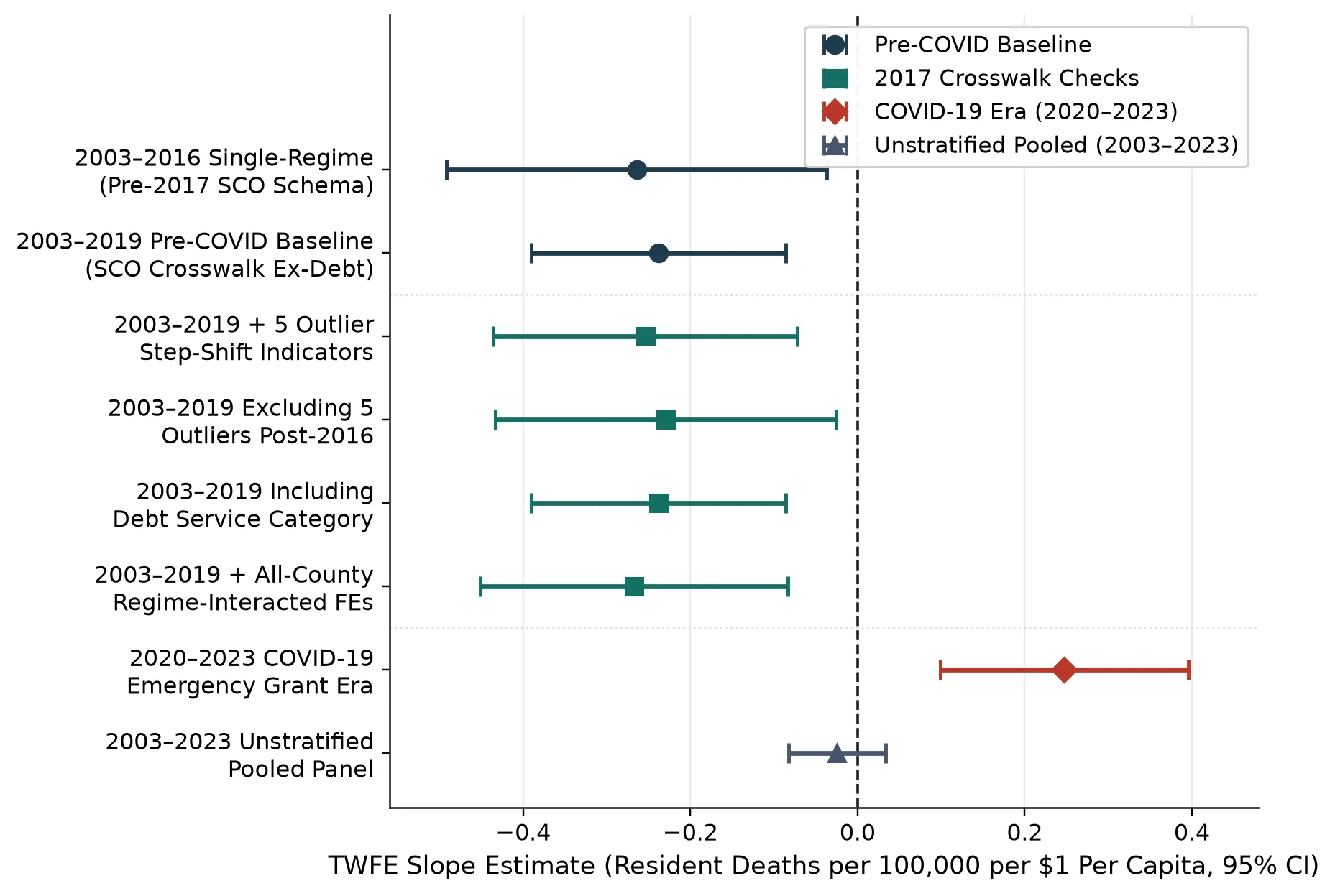
We compare all twelve regime, crosswalk, and pooled-interaction models in Table 2. In the 2003–2016 single-regime window (N = 779), where the state form never changes, the TWFE slope is -0.264 (SE = 0.116, clustered p = 0.0227; WCB p = 0.0831, WCB 95% CI [-0.573, +0.033]). Extending the pre-pandemic sample through 2019 under our primary crosswalk (N = 943) yields -0.238 (SE = 0.078, clustered p = 0.0022; WCB p = 0.0070, WCB 95% CI [-0.419, -0.083]).
| Specification & Sample Window | N (Counties) | TWFE OLS Slope (SE) | Clustered p-value | Implied Elasticity / Note |
|---|---|---|---|---|
| 2003–2016 Single-Regime ConsistentNominal $ (Pre-2017 Schema) | 779 (57) | -0.264(0.116) | 0.0227 | -0.033 |
| 2003–2016 Single-Regime ConsistentConstant 2023 $ (CPI-U) | 779 (57) | -0.154(0.087) | 0.0757 | -0.027 |
| 2003–2019 Pre-COVID SCO Crosswalk Ex-DebtNominal $ Baseline | 943 (57) | -0.238(0.078) | 0.0022 | -0.030 |
| 2003–2019 Pre-COVID SCO Crosswalk Ex-DebtConstant 2023 $ (CPI-U) | 943 (57) | -0.135(0.057) | 0.0182 | -0.024 |
| 2003–2019 + Outlier Step-Shift Indicators5 Transition Counties Post-2017 | 943 (57) | -0.254(0.093) | 0.0062 | -0.032 |
| 2003–2019 Excluding Transition OutliersDrops 5 Counties Post-2016 | 928 (57) | -0.229(0.104) | 0.0274 | -0.029 |
| 2003–2019 Crosswalk Including Debt ServiceAll 4 Post-2017 Funds | 943 (57) | -0.238(0.078) | 0.0022 | -0.030 |
| 2003–2019 + All-County Regime-Interacted FEs113 County-by-Schema FEs | 943 (57) | -0.267(0.094) | 0.0044 | -0.034 |
| 2020–2023 COVID-19 Emergency Grant Era OnlyPandemic Fiscal Regime | 220 (57) | +0.247(0.076) | 0.0011 | +0.043 |
| 2003–2023 Unstratified Pooled PanelSingle 21-Year County FE | 1,163 (57) | -0.024(0.030) | 0.4132 | -0.003 |
| 2003–2023 Stacked Regime-InteractedΔ Slope 2020–2023 + Interacted Controls | 1,163 (57) | +0.485(0.100) | <0.0001 | Pre-2020 slope = -0.238 |
| 2003–2023 County-by-Regime FE + Common ControlsΔ Slope 2020–2023 Only | 1,163 (57) | +0.605(0.098) | <0.0001 | Pre-2020 slope = -0.245 |
Across all five checks on the 2017 form change, the pre-pandemic slope stays in a narrow band between -0.229 and -0.267.
-
Outlier Step-Shift Dummies: Adding a post-2017 step-shift dummy for each of the five jump counties yields -0.254 (SE = 0.093, p = 0.0062).
-
Dropping Outlier Rows After 2016: Removing post-2016 rows for those five counties (N = 928) gives -0.229 (SE = 0.104, p = 0.0274).
-
Adding Debt Service: Including Debt Service in the 2017–2019 total leaves the slope unchanged at -0.238 (SE = 0.078, p = 0.0022).
-
Separate Post-2017 County Baselines: Giving all 57 counties separate pre-2017 and 2017–2019 baselines (113 county-by-schema effects) yields -0.267 (SE = 0.094, p = 0.0044). Because zero variation crosses the 2016–2017 line in that model, it matches the 2003–2016 slope of -0.264.
-
Inflation Adjustment: Adjusting spending and household income to constant 2023 dollars via the BLS CPI-U yields -0.135 in 2003–2019 (SE = 0.057, p = 0.0182, elasticity -0.024). Within the 2003–2016 window, the CPI-adjusted slope is -0.154 (SE = 0.087, p = 0.0757, proportional effect -0.027), reflecting the 1.38x price-level change across the period.
These five checks show that the negative 2003–2019 link is consistent across our 2017 crosswalk specifications. Dropping the five transition counties, adding step-shift indicators, or giving every county a separate post-2017 baseline keeps the 2003–2019 nominal slope between -0.229 and -0.267 (p = 0.0022 to 0.0274) and the CPI-adjusted slope at -0.135 (p = 0.0182). In the shorter 2003–2016 pre-revision window (N = 779), the nominal point estimate is similar (-0.264, clustered p = 0.0227), though its wild cluster bootstrap confidence interval spans zero (WCB p = 0.0831, 95% CI [-0.573, +0.033]) and the CPI-adjusted slope is marginal (-0.154, p = 0.0757).
Why does a simple pandemic slope interaction fail when we keep a single 21-year fixed effect per county? If a county’s health budget doubles during the pandemic, forcing one 21-year county average pulls that county’s entire baseline upward and makes pre-2020 budgets look artificially low in high-shock counties. We can see how county baselines and control slopes interact across three checks on the 2003–2023 panel (N = 1,163).
-
Common 21-Year County Baselines: Keeping one 21-year baseline per county gives +0.015 (SE = 0.073, p = 0.8394) and a crisis shift of -0.037 (SE = 0.059, p = 0.5310) under common controls. Interacting all eight covariates with the 2020 dummy produces +0.014 (SE = 0.076, p = 0.8533) and a difference of -0.055 (SE = 0.056, p = 0.3243).
-
County-by-Regime Baselines: Letting county baselines shift in 2020 under common control slopes gives a pre-pandemic slope of -0.245 (SE = 0.079, p = 0.0019) and a crisis shift of +0.605 (SE = 0.098, p < 0.0001, implied 2020–2023 slope +0.360). Letting all eight controls vary across the 2020 break produces -0.238 (SE = 0.079, p = 0.0026) and a regime difference of +0.485 (SE = 0.100, t = 4.87, p < 0.0001, 95% CI [+0.290, +0.681]).
-
Exact FWL Variance Weights (-0.0243): When we demean death rates and budgets using common 21-year county baselines, the pooled slope equals the variance-weighted sum of the two era sub-slopes. The 220 pandemic rows carry 60.8% of the residual spending sum of squares (w = 0.6083, sub-slope +0.0676, weighted term +0.0411), whereas the 943 pre-pandemic rows carry 39.2% (w = 0.3917, sub-slope -0.1670, weighted term -0.0654), summing to -0.0243.
Comparing all four cells of the 2 × 2 grid isolates the core mechanism. Separating county baselines across the 2020 break—not re-weighting the demographic controls—is what recovers the -0.238 pre-pandemic slope and the +0.485 crisis shift.
Exposure Horizons: Same-Year Links vs. Multi-Year Lags
Showing a negative same-year slope of -0.238 (p = 0.0022) from 2003 to 2019 does not prove that higher budgets lower death rates several years later. Public health programs like blood-pressure screening, maternal home visits, and clinic outreach should take years to prevent deaths, whereas standard annual regressions compare this year’s deaths to this year’s budget.5, 6, 7 If county budgets build lasting health over multi-year horizons, past spending should predict future death changes across non-overlapping windows.
To see whether the pre-pandemic link holds up over multi-year horizons, we run three sets of lag and long-difference tests. First, we test single-year lags (1, 2, 3, 5, and 8 years) and rolling multi-year averages (4-, 6-, and 9-year means) inside fixed sample windows (2011–2019, N = 498–501, and 2011–2016, N = 334). Second, we estimate stacked k-year first differences across all 16 integer horizons k ∈ {1, …, 16} from 2003 to 2019. Third, we test cross-county long-differences that separate early budget growth (2003–2010) from later death changes (2010–2016).
import numpy as np
import pandas as pd
import statsmodels.api as sm

def run_temporally_separated_long_diff(panel: pd.DataFrame, controls: list[str]) -> dict:
    """
    Regress subsequent mortality change (2010 -> 2016) on early public health
    spending change (2003 -> 2010), controlling for 2010 -> 2016 covariate changes.
    """
    y03 = panel.loc[panel["year"] == 2003].set_index("county")
    y10 = panel.loc[panel["year"] == 2010].set_index("county")
    y16 = panel.loc[panel["year"] == 2016].set_index("county")

    common = y03.index.intersection(y10.index).intersection(y16.index)
    d_ph_03_10 = y10.loc[common, "public_health_per_capita"] - y03.loc[common, "public_health_per_capita"]
    d_mort_10_16 = y16.loc[common, "mortality_rate_per_100k"] - y10.loc[common, "mortality_rate_per_100k"]
    d_ctrl_10_16 = y16.loc[common, controls] - y10.loc[common, controls]

    X = sm.add_constant(pd.concat([d_ph_03_10.rename("d_ph_03_10"), d_ctrl_10_16], axis=1))
    res = sm.OLS(d_mort_10_16, X).fit(cov_type="HC1")
    return {
        "n_counties": int(res.nobs),
        "beta": float(res.params["d_ph_03_10"]),
        "se": float(res.bse["d_ph_03_10"]),
        "p_val": float(res.pvalues["d_ph_03_10"]),
    }
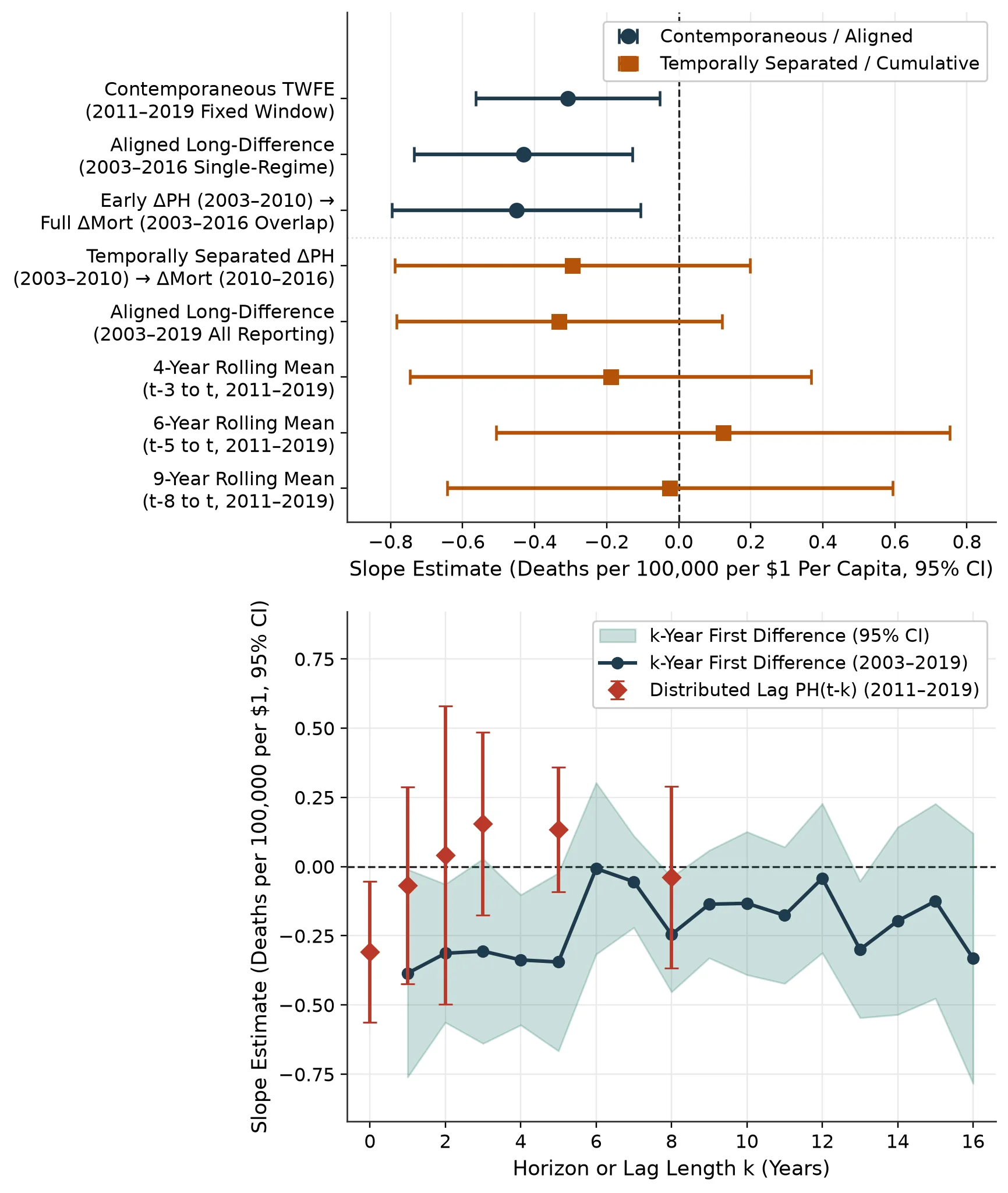
We compare the horizon and lag estimates in Figure 2 and Table 3. Four clear patterns emerge.
-
Same-Year Fixed-Window Slopes Stay Negative: If we let the sample shrink each time we add a deeper lag, we mix lag length with changing years. Holding the sample fixed at 2011–2019 (N = 498) gives a same-year slope of -0.308 (SE = 0.130, unadjusted p = 0.0178, BH-FDR q = 0.1604 across nine models), while the 2011–2016 fixed window (N = 334) gives -0.336 (SE = 0.179, p = 0.0597, FDR q = 0.1790).
-
Single Lags and Rolling Averages Fade in 2011–2019: In the 2011–2019 window, single lags at 1, 2, 3, 5, and 8 years yield -0.068 (p = 0.7075), +0.041 (p = 0.8804), +0.155 (p = 0.3570), +0.133 (p = 0.2449), and -0.039 (p = 0.8149), with FDR q = 0.9385 across all five lags. Likewise, 4-year (-0.189, p = 0.5068), 6-year (+0.123, p = 0.7017), and 9-year (-0.024, p = 0.9385) rolling averages sit near zero. In the shorter 2011–2016 sample (N = 334), the 1-year lag (-0.725, SE = 0.314, unadjusted p = 0.0210) and 8-year lag (-0.419, SE = 0.210, unadjusted p = 0.0457) have unadjusted p < 0.05. Even so, neither lag clears multiple-testing penalties (FDR q = 0.1050 and 0.1143 across five lags, or q = 0.1790 across all nine checks).
-
Stacked 16-Horizon Differences Miss Multiple-Testing Cutoffs: Across all 16 difference lengths k ∈ {1, …, 16} in 2003–2019, all 16 point estimates are negative (from -0.007 at k = 6 to -0.385 at k = 1). The 4-year difference is most precise at -0.337 (SE = 0.120, unadjusted p = 0.0049). If we test 16 horizons at once without a penalty, random noise can easily produce one low p-value. After Holm-Bonferroni or Benjamini-Hochberg adjustment, zero horizons clear the 0.05 bar (k = 4 Holm p = 0.0788, FDR q = 0.0788; k = 2, 8, 13 FDR q = 0.0814).
-
Separated Long-Differences Shrink Toward Zero: Across the 2003–2016 single-regime cross-section (N = 57), the aligned 13-year change slope is -0.432 (SE = 0.154, unadjusted p = 0.0052, Holm p = 0.0674, FDR q = 0.0674, elasticity -0.054). Regressing 2003–2016 death changes on overlapping 2003–2010 budget growth gives -0.451 (SE = 0.176, p = 0.0105). If the budget window and the death window share the years 2003 to 2010, however, a single local boom or downturn during those years moves both numbers at once. When we separate the windows so 2003–2010 budget growth predicts post-2010 death changes (2010–2016, N = 57), the slope shrinks by a third to -0.295 (SE = 0.251, p = 0.2402). Across the full 2003–2019 cross-section, the aligned 16-year change is -0.332 (SE = 0.230, p = 0.1499, N = 54) across all reporting counties and -0.591 (SE = 0.277, unadjusted p = 0.0331, N = 49) without the five 2017 jump counties.
| Horizon / Lag Specification | Sample Window | N | Slope (SE) | Unadjusted p | Adjusted q (BH-FDR) |
|---|---|---|---|---|---|
| Contemporaneous TWFE (PHt) | 2011–2019 Fixed Window | 498 | -0.308(0.130) | 0.0178 | 0.1604 |
| 1-Year Lag (PHt-1) | 2011–2019 Fixed Window | 499 | -0.068(0.182) | 0.7075 | 0.9385 |
| 2-Year Lag (PHt-2) | 2011–2019 Fixed Window | 500 | +0.041(0.274) | 0.8804 | 0.9385 |
| 3-Year Lag (PHt-3) | 2011–2019 Fixed Window | 501 | +0.155(0.168) | 0.3570 | 0.9385 |
| 5-Year Lag (PHt-5) | 2011–2019 Fixed Window | 501 | +0.133(0.115) | 0.2449 | 0.9385 |
| 8-Year Lag (PHt-8) | 2011–2019 Fixed Window | 501 | -0.039(0.167) | 0.8149 | 0.9385 |
| 4-Year Rolling Mean (PHt-3..t) | 2011–2019 Fixed Window | 498 | -0.189(0.284) | 0.5068 | 0.9385 |
| 6-Year Rolling Mean (PHt-5..t) | 2011–2019 Fixed Window | 498 | +0.123(0.321) | 0.7017 | 0.9385 |
| 9-Year Rolling Mean (PHt-8..t) | 2011–2019 Fixed Window | 498 | -0.024(0.315) | 0.9385 | 0.9385 |
| Stacked First Difference (k = 1 yr) | 2003–2019 Crosswalk | 878 | -0.385(0.191) | 0.0440 | 0.1174 |
| Stacked First Difference (k = 4 yrs) | 2003–2019 Crosswalk | 712 | -0.337(0.120) | 0.0049 | 0.0788 |
| Stacked First Difference (k = 8 yrs) | 2003–2019 Crosswalk | 492 | -0.245(0.106) | 0.0203 | 0.0814 |
| Aligned Long-Diff (2003→2016) | Cross-Section (13-yr) | 57 | -0.432(0.154) | 0.0052 | 0.0674 |
| Overlapping Early (ΔPH 03–10 → ΔMort 03–16) | Cross-Section (Overlap) | 57 | -0.451(0.176) | 0.0105 | N/A |
| Temporally Separated (ΔPH 03–10 → ΔMort 10–16) | Cross-Section (Separated) | 57 | -0.295(0.251) | 0.2402 | N/A |
| Aligned Long-Diff (2003→2019 All Reporting) | Cross-Section (16-yr) | 54 | -0.332(0.230) | 0.1499 | 0.2725 |
| Aligned Long-Diff (2003→2019 Excl. 5 Outliers) | Cross-Section (16-yr) | 49 | -0.591(0.277) | 0.0331 | N/A |
These horizon checks set a clear boundary on what the pre-pandemic panel can and cannot prove. The data show a consistent same-year within-county link (-0.238 in 2003–2019, -0.264 in 2003–2016) and a negative aligned 2003–2016 cross-county slope (-0.432). Once we separate the time windows or penalize for testing 16 horizons at once, however, the panel cannot pin down a multi-year causal lag.
Cause-Specific Deaths, County Size, and Time Ordering
What if our pre-pandemic budget slope were simply picking up general county wealth or hospital trauma care? If it were, we would see the slope across every cause of death, including car crashes and falls. To see whether the pre-2020 slope tracks conditions that public health departments target, we split CDPH records by cause of death, county size, and pre/post-ACA eras (Table 4).
| Diagnostic Dimension & Specification (2003–2019) | N (Counties) | TWFE OLS Slope (SE) | Clustered p-value | Share / Elasticity Note |
|---|---|---|---|---|
| Preventable Mortality (9-Cause Composite) | 923 (56) | -0.284(0.093) | 0.0022 | Elasticity -0.072 |
| Preventable Mortality (5-Cause Complete-Case) | 719 (47) | -0.099(0.061) | 0.1033 | Elasticity -0.025 |
| Diseases of the Heart (HTD) | 923 (56) | -0.115(0.042) | 0.0066 | 48.4% of all-cause slope |
| Cerebrovascular Disease / Stroke (STK) | 814 (53) | -0.024(0.025) | 0.3319 | Elasticity -0.045 |
| Chronic Lower Respiratory Disease (CLRD) | 868 (54) | -0.012(0.020) | 0.5422 | Elasticity -0.022 |
| Diabetes Mellitus (DIA) | 723 (48) | -0.010(0.011) | 0.3941 | Elasticity -0.037 |
| Influenza and Pneumonia (PNF) | 725 (49) | -0.009(0.016) | 0.5736 | Elasticity -0.039 |
| Unintentional Injuries (INJ) | 857 (55) | -0.002(0.015) | 0.9009 | Elasticity -0.004 |
| Large Urban Counties (Population > 500,000) | 251 (16) | -0.259(0.055) | <0.0001 | Elasticity -0.030 |
| Rural & Medium Counties (Population ≤ 500,000) | 692 (43) | -0.242(0.098) | 0.0136 | Elasticity -0.032 |
| 2003–2009 Pre-ACA Enactment Subperiod | 388 (57) | -0.648(0.210) | 0.0020 | Elasticity -0.081 |
| 2010–2019 Post-ACA Enactment Subperiod | 555 (57) | -0.216(0.144) | 0.1345 | Elasticity -0.028 |
| Pooled Post-2010 Interaction (PH × I[t ≥ 2010]) | 943 (57) | +0.0003(0.101) | 0.9974 | No structural break in 2010 |
Three findings clarify what drives the 2003–2019 estimates.
-
Heart Disease Drives Nearly Half of the Slope: Diseases of the heart (HTD, N = 923 across 56 counties) show a slope of -0.115 deaths per 100,000 per dollar (SE = 0.042, p = 0.0066, elasticity -0.058). That single cause makes up 48.4% (-0.11508 / -0.23790) of the all-cause gradient. Our 9-cause preventable composite sums non-suppressed counts across heart disease, stroke, CLRD, diabetes, flu/pneumonia, liver disease, hypertension, kidney disease, and suicide, yielding -0.284 (SE = 0.093, p = 0.0022). If we require complete cases across all five leading causes at once (HTD, STK, CLRD, DIA, and PNF), privacy rules drop 224 rural county-years (N = 719, 47 counties) and shrink the slope to -0.099 (SE = 0.061, p = 0.1033). Meanwhile, unintentional injuries (INJ, N = 857 across 55 counties)—which reflect highway traffic and trauma care rather than health department outreach—sit near zero at -0.002 (SE = 0.015, p = 0.9009).
-
Urban and Rural Counties Match Closely: The 2003–2019 slope is -0.259 (SE = 0.055, p < 0.0001) in the 16 large urban counties above 500,000 residents (N = 251) and -0.242 (SE = 0.098, p = 0.0136) in the 43 smaller counties (N = 692). Dropping each of the 10 largest counties one by one keeps the slope between -0.230 (without Santa Clara, p = 0.0034) and -0.246 (without Sacramento, p = 0.0030; dropping Los Angeles gives -0.238, SE = 0.083, p = 0.0039). Splitting 2003–2009 (-0.648, SE = 0.210, p = 0.0020) and 2010–2019 (-0.216, SE = 0.144, p = 0.1345) widens the error bars in each shorter window. Even so, a pooled post-2010 interaction (N = 943) is +0.0003 (SE = 0.101, p = 0.9974), showing no regime break after the 2010 Affordable Care Act.
-
Future Budgets Do Not Predict Past Deaths: If next year’s health budget already predicted this year’s deaths, our regression would just be capturing a pre-existing county trend. In our lead check on 2003–2019 (N = 888), current spending stays negative (-0.198, SE = 0.081, p = 0.0147) while next year’s spending does not significantly predict current deaths (-0.116, SE = 0.102, p = 0.2564). In the reverse direction, regressing current budgets on last year’s death rate in 2003–2019 gives -0.048 dollars per death per 100,000 (SE = 0.022, p = 0.0270), because local downturns raise death rates while squeezing county tax revenue. During 2020–2023 (N = 220), that 1-year reverse-lag slope is -0.269 (SE = 0.180, p = 0.1385, 95% CI [-0.622, +0.085]), which is too noisy to separate lagged budget responses from same-year crisis waves.
Together, the cause-specific and timing checks clarify the scope of the pre-pandemic link. The 2003–2019 within-county slope is concentrated in chronic heart-disease deaths (-0.115, p = 0.0066) rather than unintentional injuries (-0.002, p = 0.9009) and holds across both urban (-0.259) and rural (-0.242) counties. While the 1-year reverse-lag slope (-0.048, p = 0.0270) goes in the opposite direction of crisis-style positive budget targeting, the noisy 1-year lead estimate (-0.116, p = 0.2564) means these same-year regressions reflect within-county associations rather than isolated causal effects.
Practical Checklist for Multi-Decade Panel Regressions
Four diagnostic steps keep long panel regressions from hiding accounting shifts or crisis regime breaks.
-
Interact Unit Baselines Across Crisis Eras: Without separate unit baselines across a crisis break, high-variance emergency aid can dominate the pooled slope (+0.485 shift, p < 0.0001). Always pair a regime-interaction test with Frisch-Waugh-Lovell variance weights (60.8% pandemic weight vs. 39.2% pre-pandemic weight) when a major shock hits the panel.8, 9
-
Check Accounting Transitions County by County: Inspect cross-county correlations (r = 0.996 in total dollars, r = 0.916 per person at the 2016–2017 line) and flag unit jumps over 50%. Confirm that giving every county a separate post-revision baseline (-0.267, p = 0.0044) matches the single-form slope (-0.264, p = 0.0227).
-
Recode Late Filings Before Running Regressions: Separate true zero spending from late or unfiled state forms (7 post-2016 county-years in Fresno, Humboldt, and Mendocino) before demeaning within counties.
-
Test Non-Overlapping Horizons and Adjust for Multiple Tests: Report single-year lags, non-overlapping long-differences, and multiple-testing q-values (Holm and Benjamini-Hochberg FDR) across all tested horizons. That discipline keeps same-year correlations from being overstated as multi-year causal paybacks.10, 11, 12
References
- California State Controller's Office. (2024). Counties Financial Data: By the Numbers (Dataset ID: uctr-c2j8, FY 2002–03 through FY 2022–23). Sacramento, CA: California Open Data Portal. ↑
- California Department of Public Health. (2024). Death Profiles by County, 1999–2023. Sacramento, CA: CDPH Center for Health Statistics and Informatics. ↑
- Cameron, A. C., Gelbach, J. B., & Miller, D. L. (2008). Bootstrap-based improvements for inference with clustered errors. Review of Economics and Statistics, 90(3), 414–427. doi:10.1162/rest.90.3.414 ↑
- Roodman, D., Nielsen, M. Ø., MacKinnon, J. G., & Webb, M. D. (2019). Fast and wild: Bootstrap inference in Stata using boottest. The Stata Journal, 19(1), 4–60. doi:10.1177/1536867X19830877 ↑
- Mays, G. P., & Smith, S. A. (2011). Public health system performance and community health outcomes. American Journal of Preventive Medicine, 41(6), 546–551. ↑
- Brown, T. T. (2014). How effective are public health departments at preventing mortality? Health Economics, Policy and Law, 9(3), 287–304. ↑
- Brown, T. T. (2016). Returns on investment in California county departments of public health. American Journal of Public Health, 106(8), 1477–1482. ↑
- Maani, N., & Galea, S. (2020). COVID-19 and underinvestment in the public health infrastructure of the United States. The Milbank Quarterly, 98(2), 250–259. ↑
- Dave, D. M., Friedson, A. I., McNichols, D., & Sabia, J. J. (2023). Associations between county-level public health expenditures and community health planning activities with COVID-19 incidence and mortality. Public Health, 225, 84–92. ↑
- Benjamini, Y., & Hochberg, Y. (1995). Controlling the false discovery rate: A practical and powerful approach to multiple testing. Journal of the Royal Statistical Society: Series B (Methodological), 57(1), 289–300. doi:10.1111/j.2517-6161.1995.tb02031.x ↑
- Holm, S. (1979). A simple sequentially rejective multiple test procedure. Scandinavian Journal of Statistics, 6(2), 65–70. ↑
- Wooldridge, J. M. (2010). Econometric Analysis of Cross Section and Panel Data (2nd ed.). Cambridge, MA: MIT Press. ↑
Cite this article
Cholette, V. (2026, October 26). Public Health Spending: When Crisis Aid Flips the Sign. Too Early To Say. https://tooearlytosay.com/research/health-policy/public-health-spending-regime-shifts/