The statement "Hispanic neighborhoods have higher food insecurity" would draw little debate. USDA data consistently shows Hispanic households experience food insecurity at roughly 1.6 times the national rate: 21.9% in 2023 compared to 13.5% overall (Rabbitt et al., 2024).

But consider what we find when we look deeper:

• 29 census tracts with high Asian populations and low vehicle ownership fall in the top two vulnerability quintiles, more tracts than any Hispanic-defined group
• The single tract with the most geographic barriers has the highest vulnerability score (0.437) but the lowest SNAP participation (5.3%)
• Hispanic + children + low education compounds to 21.2% SNAP participation, yet Hispanic identity alone doesn't predict vulnerability

The problem with single-variable analysis is that it flattens complexity. "Hispanic = vulnerable" ignores that a high-income Hispanic professional in Palo Alto faces different barriers than a Hispanic single mother in East San Jose.

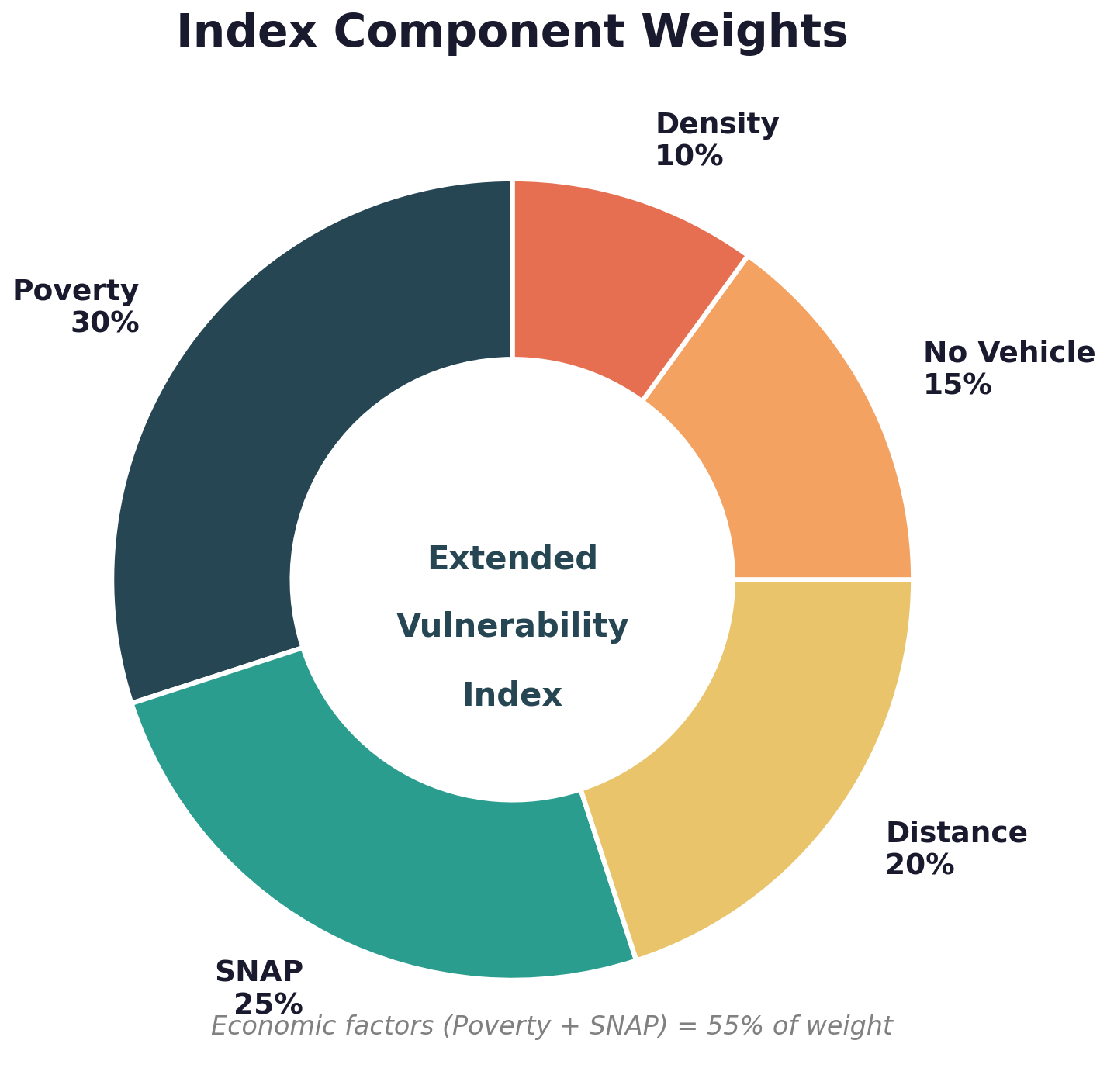
Given this complexity, we can build an Extended Vulnerability Index that combines multiple components (poverty, SNAP participation, grocery distance, vehicle access, and population density) with explicit weights, validated against outcomes, and tested for robustness.

What we discover: Intersections matter. Geography matters. And the index reveals patterns invisible to demographic crosstabs.

In this post, we explain how to construct a neighborhood-level vulnerability index, when to use one (and when not to), and what this one reveals about food security in Santa Clara County.

Why Build a Composite Index?

The Problem with Single Variables

Food insecurity is multidimensional:

• Economic: Can families afford food?
• Geographic: Can they access stores?
• Mobility: Can they get there?
• Social: Do they face discrimination or language barriers?

Single-variable analysis (poverty rate alone, distance to grocery alone) captures one dimension while ignoring others. A tract could have low poverty but terrible transit (mobility barrier), high poverty but excellent store access (economic barrier only), or moderate everything but compounding disadvantages.

When to Use a Composite Index

We can use a composite index when:

1. The outcome is multidimensional (food security involves economics, geography, mobility, social factors)
2. The goal is to rank or prioritize (which 20 neighborhoods need intervention first?)
3. We need to capture compounding effects (vulnerabilities that multiply)
4. Policy requires tractable targeting (resources can't be deployed everywhere at once)

We typically want to avoid a composite index when:

1. Causal identification is needed (indices conflate predictors; use regression for causation)
2. A single dimension dominates (if 95% of variation is poverty, just use poverty)
3. Transparency matters more than precision (black-box indices obscure what's driving scores)
4. Components are highly correlated (double-counting the same thing)

The Santa Clara County Context

We needed an index because:

• The county has zero food deserts by USDA definition (geography isn't the barrier)
• But 4.7x variation in SNAP rates exists across tracts (something drives disparities)
• Policy question: Which specific neighborhoods need intervention?
• Single variables couldn't answer this: poverty alone missed mobility barriers, and distance alone missed economic barriers

Building the Extended Vulnerability Index

Theoretical Foundation

Our index draws on the WHO Social Determinants of Health framework (Solar & Irwin, 2010), which identifies structural determinants (socioeconomic position, education, income), intermediary determinants (material circumstances, behaviors), and health system factors (access, quality).

For food security, we translate this to five components:

Why These Weights?

Weights are the most contested part of any composite index. Here's our reasoning:

Economic components (55% total): Literature consensus holds that affordability dominates food security. The USDA's annual food security reports (Rabbitt et al., 2024) consistently show that households below the federal poverty line experience food insecurity at rates 3-4 times higher than the general population: 38.7% of households below the poverty line were food insecure in 2023, compared to 13.5% overall.

Geographic (20%): Important but secondary in urban counties. Distance matters more in rural areas.

Mobility (15%): Captures transit-dependent populations often missed by distance measures.

Density (10%): Contextual adjustment. Dense areas have more options; sparse areas have fewer.

The key insight: We tested alternative weights (see Validation section). Rankings are robust; the exact weights matter less than including the right components.

Validating the Index

Criterion Validity: Does It Predict What It Should?

An index is only useful if it correlates with outcomes it should predict.

We use SNAP participation as our validation criterion:

• Spearman correlation: r = 0.83 (p < 0.001)
• Strong positive relationship: higher EVI → higher SNAP rates
• This makes sense: tracts with economic + geographic barriers should have more households needing food assistance

To interpret this correlation: Cohen (1988) established widely-used benchmarks where r < 0.30 indicates a weak relationship, 0.30-0.50 is moderate, and r > 0.50 is strong. For criterion validity specifically, Schober et al. (2018) suggest correlations above 0.70 represent "strong" validity. Our r = 0.83 falls well into this strong range, suggesting the index genuinely captures food security vulnerability rather than measuring something else entirely.

Sensitivity Analysis: Are Rankings Robust?

The biggest criticism of composite indices: "The weights were selected to get a desired answer."

We tested five alternative weighting schemes. All schemes produce Spearman r > 0.91 with baseline rankings. Top 20% agreement exceeds 96%.

Why does r > 0.91 matter? In sensitivity analysis for composite indices, we're asking whether rankings stay stable when we change our assumptions. Paruolo et al. (2013) demonstrate that even "seemingly innocent modifications" to index construction can produce "remarkable changes in ranking." An r > 0.90 between alternative specifications indicates the rankings are highly stable; the same neighborhoods appear in the top quintile regardless of which reasonable weighting scheme we apply. This isn't always the case: poorly constructed indices can show dramatic rank reversals with minor weight adjustments.

What this means: The same tracts end up in the highest vulnerability quintile regardless of exact weights. Our index is robust to reasonable methodological choices.

What the Index Reveals

Finding 1: Geography Doesn't Equal Need

The single tract with the most geographic barriers (1.29 miles to nearest grocery, 40% no-vehicle households):

• Highest vulnerability score: 0.437
• Lowest SNAP participation: 5.3%

Geographic isolation creates barriers, but the population there either doesn't qualify for SNAP, doesn't know about it, or faces other barriers to enrollment. High vulnerability doesn't automatically mean high program uptake.

What we conclude: This tract needs outreach, not new stores.

Finding 2: Intersections Matter More Than Single Identities

When we analyze intersectional groups (combinations of demographic and vulnerability characteristics), hidden patterns emerge:

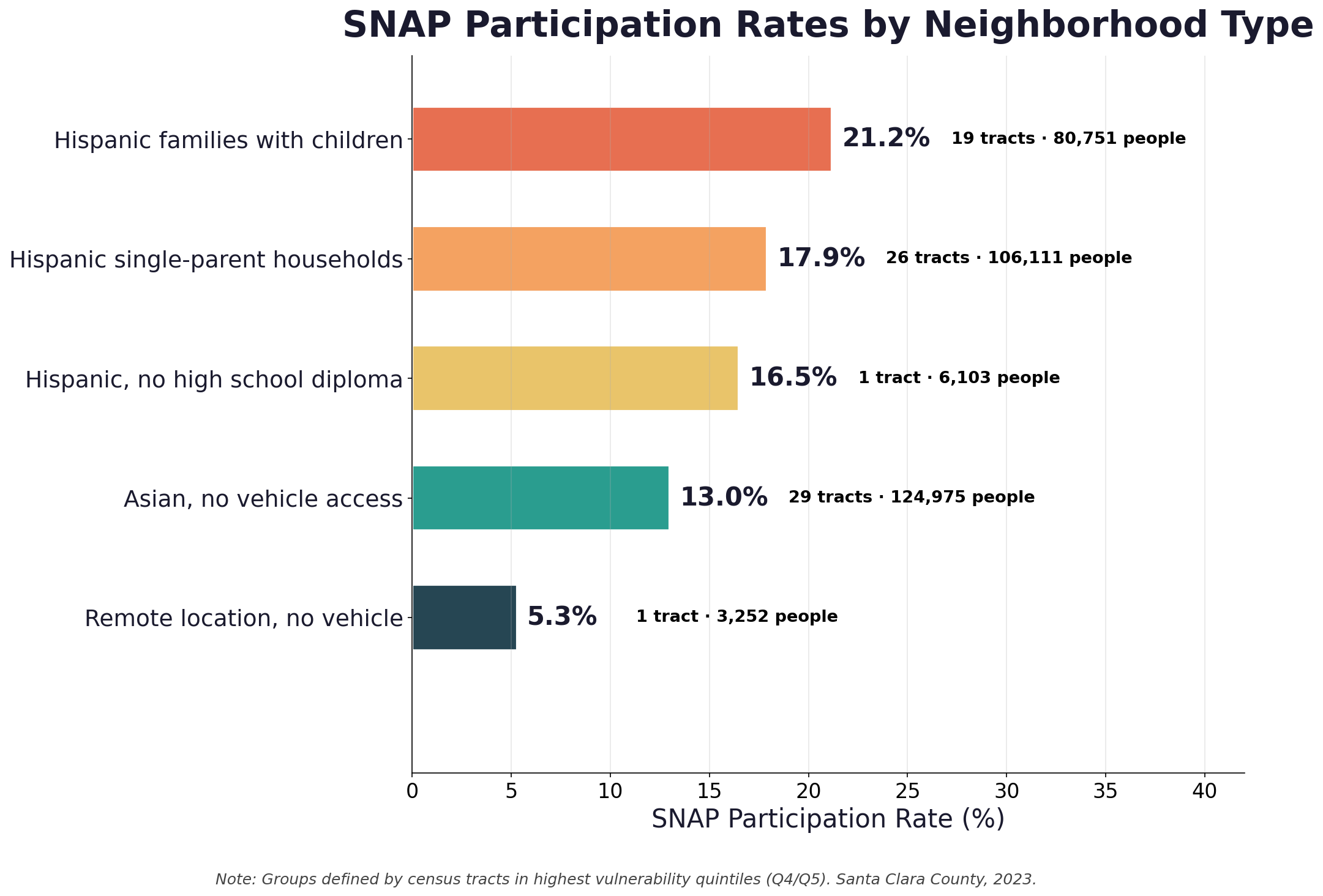
The High Asian + Low Vehicle group has 29 tracts, more than any Hispanic-defined group. This group is invisible to standard demographic analysis. Asian populations are often stereotyped as having low food insecurity, but transit-dependent Asian households (elderly, recent immigrants, low-income) face real barriers. Cultural food access adds another layer: ethnic grocery stores may not accept SNAP.

What we observe is that Hispanic identity alone doesn't predict vulnerability. It's Hispanic + children + low education + single parent that compounds to extreme SNAP rates (21.2%). A Hispanic software engineer in Cupertino isn't food insecure. A Hispanic single mother with three kids and no high school diploma in East San Jose is.

Finding 3: The Q5 Profile

What characterizes the highest-vulnerability tracts (Q5)?

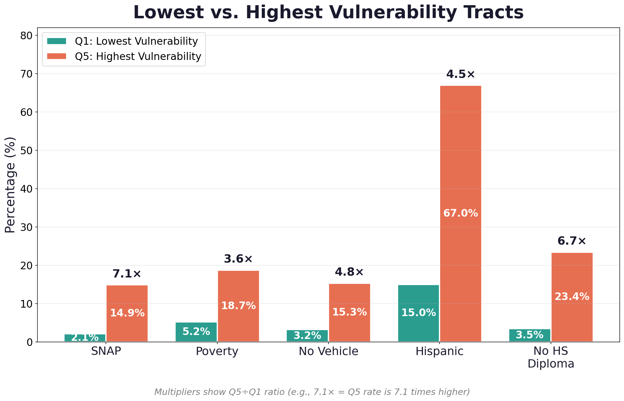
• SNAP rates are 7.1× higher in Q5 tracts
• Hispanic population share is 4.5× higher
• The percent without a high school diploma is 6.7× higher

We find Q5 tracts cluster geographically: East San Jose (18 tracts, ~72,000 residents), South County/Gilroy (7 tracts, ~28,000 residents), and North San Jose industrial areas (3 tracts, ~12,000 residents).

When to Use This Index (And When Not To)

Where the EVI Adds Value

Program Targeting: "Which 20 tracts should receive Spanish-language SNAP outreach first?" The EVI ranks tracts; pick a threshold and deploy resources.

Resource Allocation: "How should $1M in food assistance grants be distributed?" We can weight by EVI × population to prioritize high-need, high-population areas.

Monitoring Over Time: "Are vulnerable neighborhoods getting better or worse?" Track EVI changes to identify deteriorating areas.

Cross-Jurisdiction Comparison: "How does Santa Clara compare to Alameda County?" Our standardized index enables apples-to-apples comparison.

Where the EVI Falls Short

Not Causal: The index shows where vulnerability concentrates, not why. High EVI could result from labor market conditions, housing costs, discrimination, or historical disinvestment. Policy needs to address causes, not just correlations.

Aggregation Hides Variation: The index describes the average tract, missing within-tract heterogeneity. Some households in a moderate-EVI tract have cars and high incomes; others are transit-dependent with no savings.

Components Are Correlated: Poverty and SNAP participation correlate at r = 0.71. Economic disadvantage is partially double-counted. We acknowledge this is intentional (both capture food security risk) but it inflates apparent precision.

Static Snapshot: 2023 data doesn't capture seasonal variation, economic shocks, or program changes.

Final Thoughts

The EVI is a useful heuristic for prioritization, not a precise measurement of food insecurity. It answers "where should we look first?" not "exactly how food insecure is this tract?"

It works well for targeting. It's less suited for causal claims.

For those building similar indices, three methodological points bear emphasis. First, any composite index should correlate with outcomes it claims to predict; validation is not optional. Second, sensitivity analysis is mandatory: if findings depend on arbitrary weight choices, they're not findings. Third, intersectional analysis requires adequate sample sizes; our analysis required minimum 10 tracts per group, and smaller samples produce unstable estimates.

Methodology Note

Data Sources: Census ACS 5-Year Estimates (2019-2023), Google Maps Places API (6,613 validated grocery stores), Census TIGER/Line shapefiles

Sample: 408 census tracts, Santa Clara County, California

Index Construction: Min-max normalization, weighted linear combination, quintile classification

Validation: Criterion validity (Spearman r = 0.83 with SNAP participation), sensitivity analysis (5 alternative weighting schemes, all r > 0.91)

Reproducibility: Full code and data sources available on GitHub.

References

Cohen, J. (1988). Statistical power analysis for the behavioral sciences (2nd ed.). Lawrence Erlbaum Associates.

Paruolo, P., Saisana, M., & Saltelli, A. (2013). Ratings and rankings: Voodoo or science? Journal of the Royal Statistical Society: Series A, 176(3), 609-634.

Rabbitt, M.P., Reed-Jones, M., Hales, L.J., & Burke, M.P. (2024). Household food security in the United States in 2023 (Report No. ERR-337). U.S. Department of Agriculture, Economic Research Service.

Schober, P., Boer, C., & Schwarte, L.A. (2018). Correlation coefficients: Appropriate use and interpretation. Anesthesia & Analgesia, 126(5), 1763-1768.

Solar, O., & Irwin, A. (2010). A conceptual framework for action on the social determinants of health (Social Determinants of Health Discussion Paper 2). World Health Organization.