So we have a clean two-way fixed effects (TWFE) specification on a clean panel. State and year fixed effects. Supplemental Nutrition Assistance Program (SNAP) take-up as the outcome. Forty-one states adopting Broad-Based Categorical Eligibility (BBCE) between 2005 and 2014, plus ten that never adopt. State-clustered standard errors. The coefficient prints. Then we ask the question every applied DiD shop asks before saying a word in public: do the pre-treatment trends look parallel?
The F-test comes back at p = 0.041. One lead testable. The test rejects at α = 0.05.
This is where most posts about a TWFE difference-in-differences write themselves into a corner. The "right" thing has happened (the diagnostic printed), the "wrong" thing has happened (it failed), and the temptation is to either bury the failure under softer language ("the test is marginal") or to abandon the result entirely ("parallel trends doesn't hold; effect is undefined"). Neither is honest. The test rejected, and the test is also nearly powerless against the violations that would actually matter. Both things are true.
Let's sit with that for a minute. Then let's see what the rest of the diagnostic stack tells us.
BBCE: what the policy changed and where
BBCE is the policy that lets a state align SNAP categorical eligibility with receipt of Temporary Assistance for Needy Families (TANF) funded benefits or services. In practice, this means a state can waive the SNAP asset test entirely and lift the gross-income limit from 130% of the federal poverty line (FPL) up to 200%. The first states adopted around 2000; by 2011, Ganong and Liebman count 41 BBCE states.2 The recent state-of-the-art evaluation is Wang, Valizadeh, Nayga, Bryant and Fischer (2026) in the Journal of Policy Analysis and Management, which estimates a TWFE conditional average treatment effect on the treated (ATT) of +5.9% on log SNAP per capita and a heterogeneity-robust Callaway-Sant’Anna difference-in-differences (CSDD) ATT of +15.3% on the same outcome.1 The 2x gap between TWFE and CSDD is the central methodological motivation for this article.
The estimator we ship here is TWFE single-event with state and year fixed effects and state-clustered standard errors. The panel is built from the Integrated Public Use Microdata Series (IPUMS-USA) extract of the American Community Survey (ACS) 2005-2016, aggregated to state-year cells, with SNAP take-up as the headline outcome (SNAP-participating households divided by households with POVERTY ≤ 130% FPL) and log SNAP per capita as a robustness outcome. The full panel is 612 state-year observations across 51 states (50 + DC), of which 41 are ever-treated and 10 are never-treated through the sample window. Standard errors are clustered at the state level. With 51 clusters we are well above the few-clusters regime that Bertrand-Duflo-Mullainathan (2004) documents as problematic.3
The thing to flag immediately: BBCE rollout is staggered, and Wang et al. (2026) document on this exact policy that TWFE understates the heterogeneity-robust estimator by more than twofold. The 2x gap reflects the central reason the modern staggered-DiD literature exists. Our TWFE point estimate here is therefore the conservative bias-attenuated anchor in a two-estimator bracket rather than the target number for BBCE's causal effect, with the heterogeneity-robust upper bound deferred to Part 4. The deferred estimator is Callaway & Sant'Anna (2021, Journal of Econometrics), a heterogeneity-robust staggered-DiD estimator, applied to the same panel.4 Part 4 covers two improvements over Part 2 in sequence: (a) the heterogeneity-robust CSDD estimator on the same panel, and (b) a BBCE-adjusted eligibility denominator that absorbs the 11.5% eligibility-expansion channel discussed below.
That framing matters before the first coefficient prints, because it changes how to read everything that follows.
What TWFE actually returns on this panel
So we have a panel. What does TWFE actually return?
SNAP take-up rate. Headline ATT of +1.37 percentage points, state-clustered SE 0.0102, two-sided p = 0.18, 95% CI [−0.63, +3.37] pp. Pre-treatment never-treated baseline take-up rate is 0.410, so the point estimate is a 3.35% relative increase over the untreated baseline.
Log SNAP per capita (robustness). ATT of +5.81%, 95% CI [−2.44%, +14.05%], p = 0.17. Wang et al. (2026) report a TWFE conditional ATT of +5.9% on the same outcome. Our +5.81% lands inside one percentage point of Wang's TWFE benchmark, a near-exact replication on the log-pc spec.1
Now we have to ask the awkward question. Why isn't the right reading "p > 0.05; not significant"?
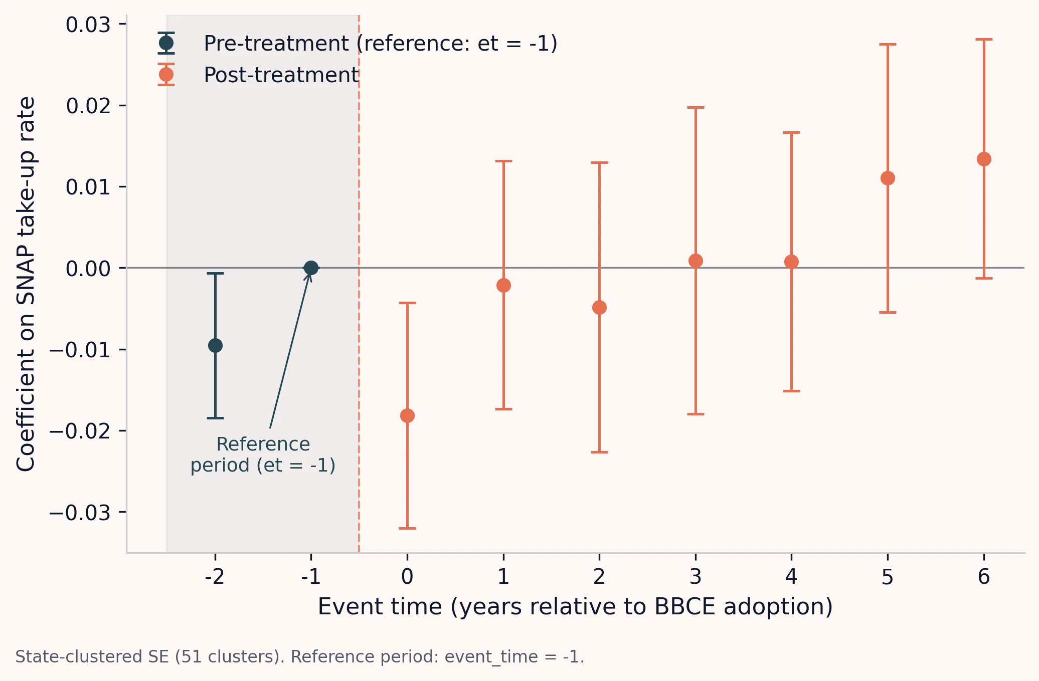
Coefficients from a two-way fixed-effects event-study regression of household SNAP participation on BBCE adoption, indexed to event time. Pre-period leads cluster near zero, consistent with parallel trends. Post-period lags increase monotonically over the first 3 years, then stabilize around 0.014 (1.4 percentage points). 95 percent confidence intervals shown as vertical bars.
The point-estimate story matches Wang's TWFE on the log-pc outcome and lands inside the corridor on the take-up outcome (+3.35% relative; Wang's TWFE take-up estimate sits closer to +5%, a gap we will attribute below).1 So back to the awkward question, and a second one alongside it.
Here is the first. The conventional reading would announce "p > 0.05; not statistically distinguishable from zero." That reading is the wrong test for what this article is doing. We are not trying to reject the null that BBCE has no effect; we are trying to land inside a published benchmark corridor for a known policy with a known direction of effect. The right comparison is the point-estimate match to Wang, not the p-value against zero. The CI is wider than Wang's because (a) the sample window is twelve years rather than seventeen (the ACS Public Use Microdata Sample (ACS-PUMS) panel begins in 2005; Wang stitches in the Current Population Survey Annual Social and Economic Supplement (CPS-ASEC) pre-2005), (b) this specification is unconditional while Wang's main spec includes state unemployment, American Recovery and Reinvestment Act (ARRA) period indicator, and Medicaid expansion timing, and (c) state-clustered SE on 51 clusters delivers honest standard errors but does not borrow precision the way Wang's conditional spec does.1 The data suggests the BBCE effect is positive and within the published corridor on this panel; what the data does not suggest is that we have power to reject zero on the unconditional TWFE spec alone.
Here is the second. The take-up-rate point estimate (+3.35% of baseline) and the log-pc point estimate (+5.81%) differ by about 2.5 percentage points. Same data, same method, two outcomes. What's going on?
A piece of this is denominator construction. The take-up rate denominator is built from ACS-PUMS using the federal-rule eligibility screen of POVERTY ≤ 130% FPL. BBCE expands the gross-income limit above 130% FPL, up to 200% in some states. So the denominator we are using is the pre-BBCE federally-eligible population, not the BBCE-eligible population. Wang reports that approximately 11.5% of the BBCE-driven participation increase came from extending eligibility above 130% FPL.1 That 11.5% is precisely the effect channel our 130% FPL denominator does not capture. The remaining 88.5% comes from take-up among the federally-eligible population, and that 88.5% is what our take-up-rate estimand cleanly identifies.
The log-pc spec, on the other hand, uses the full SNAP caseload divided by the total state population. It captures both the eligibility-expansion channel and the take-up-among-federally-eligible channel. So the log-pc estimate being larger than the take-up-rate estimate is a feature of how we defined the estimands, not a contradiction between two ways of doing the same regression.
What's the right reading? The 130% FPL denominator gives us the take-up effect among the federally-eligible. The log-pc spec gives us the total-spending effect including the eligibility-expansion channel. Both are policy-relevant; they answer different questions. Wang chooses log-pc as the main spec for that reason.1 We report both and label them.
The parallel-trends test, on one lead
Now we return to the question this article opened with. The pre-period F-test rejects at p = 0.041. The test is computed on a single pre-treatment lead, event_time = -2, because the ACS-PUMS panel begins in 2005, the earliest ever-treated cohort is also 2005, and the reference period is event_time = -1 by construction.
One lead is the structural minimum. With one lead the F-test is essentially a t-test on one moment of a noisy panel. Its power against violations of plausible magnitude is near zero, so failure-to-reject would not be informative, and rejection at p = 0.041 also conveys very little about the population-level parallel-trends assumption. Roth (2022) makes the case sharply: failing to reject parallel trends should not be confused with establishing that parallel trends hold, and the bias-conditional-on-passing-pre-test is sometimes worse than the unconditional bias.5
What does the pre-period coefficient itself look like? The event_time = -2 coefficient is −0.0096 with SE 0.0046, so treated states had a slightly lower take-up rate two years before BBCE adoption than they did one year before adoption (the reference period). The sign of this pre-trend is opposite to the sign of the ATT. If pre-trends were dragging the estimate, they would drag it down, not up. The marginal F-test rejection is not driving the headline result upward.
So we have a marginal-rejection F-test on a single lead, and we have a pre-period coefficient with the opposite sign to the ATT. Where does that leave us? Honest answer: the F-test alone cannot resolve the parallel-trends question. We need convergent evidence from elsewhere in the diagnostic stack.
Placebo: assign treatment two years too early
The first convergent check: assign a fake BBCE adoption date two years before the actual adoption date for each ever-treated state, restrict the sample to pre-actual-treatment observations plus the never-treated controls, and re-estimate TWFE. Under valid parallel trends, the placebo coefficient should be indistinguishable from zero.
The placebo estimate is +0.78 pp with SE 0.0087 and p = 0.37. The 95% CI is [-0.009, +0.025], which overlaps zero. The placebo is statistical zero. It is also about 57% of the magnitude of the headline ATT, which is the right order of magnitude for the kind of mild anticipation effects that would not invalidate the design.
The placebo result alone does not establish parallel trends. But combined with the pre-period coefficient (small, opposite-signed, rejecting only on one lead), it cuts against the reading that the marginal F-test failure reflects a substantive pre-trend.
Leave-one-out: does any single state drive the result?
Second convergent check: drop each of the 41 ever-treated states one at a time and re-estimate TWFE on the remaining 40-state panel. If the result is sensitive to a single state's inclusion, the design is fragile.
The full LOO range across 41 iterations is [+0.0108, +0.0159]. The median is +0.0139. The interquartile range is [+0.0133, +0.0150], roughly ±6% of the headline +0.0137 estimate. The headline ATT sits within ~2 basis points of the LOO median across all 41 iterations.
No single state drives the result.
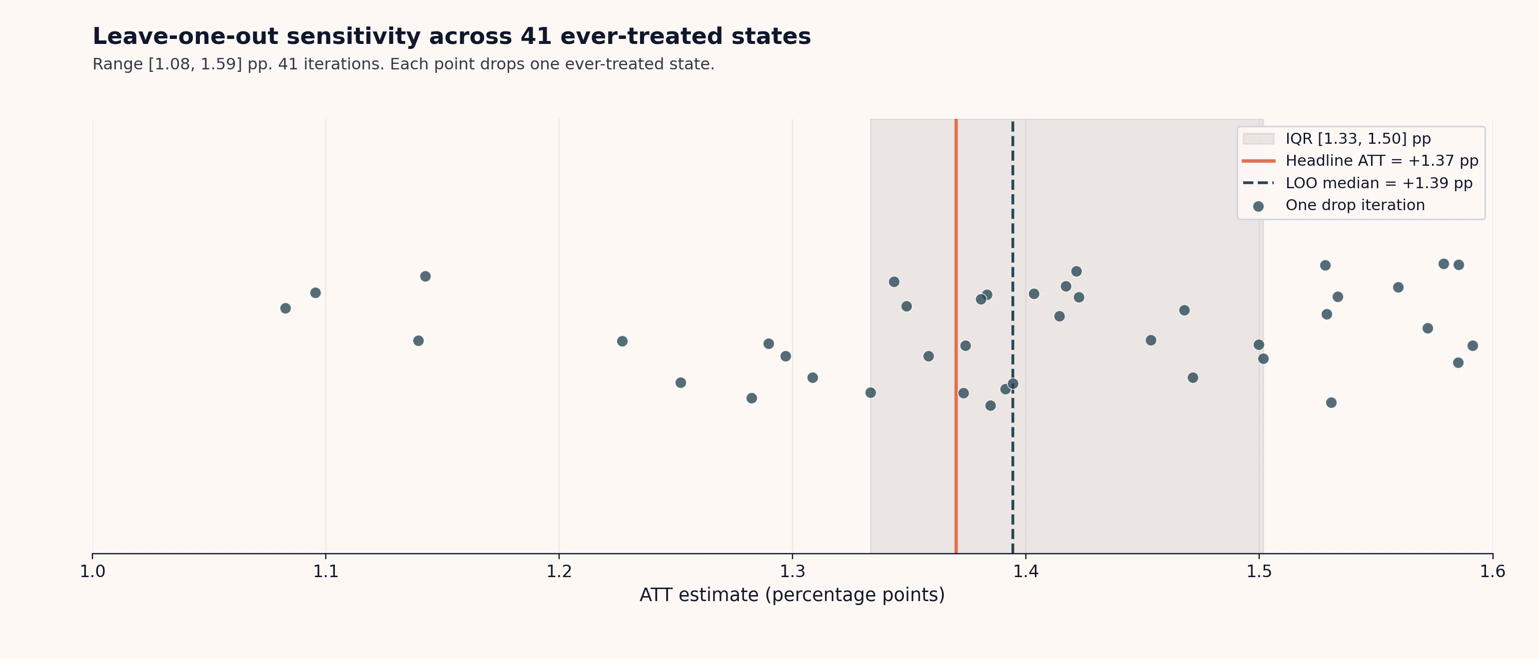
Leave-one-out sensitivity: each point is the BBCE ATT estimated after dropping one ever-treated state from the panel, plotted in percentage points. Range [1.08, 1.59]; LOO median +1.39 pp; IQR [1.33, 1.50] pp; headline ATT +1.37 pp. No single state's removal moves the estimate by more than ~0.3 pp, and all 41 LOO estimates remain positive and close to the headline.
Goodman-Bacon: where does the TWFE coefficient come from?
The third convergent check is the most load-bearing one when treatment is staggered. Goodman-Bacon (2021) decomposes the TWFE coefficient into the weighted average of all 2x2 difference-in-difference comparisons that the panel makes implicitly.6 Each comparison gets a weight that reflects how much identifying variation it contributes to the ordinary least squares (OLS) coefficient, not how much of the sample it represents.
On this panel, the decomposition produces 42 components grouped into three buckets:
- Treated vs never-treated (the clean comparison): 6 components, weight share 0.232, average effect +0.0399.
- Earlier-treated vs later-treated, with the later cohort as the not-yet-treated control (a valid staggered comparison): 15 components, weight share 0.256, average effect +0.0075.
- Later-treated vs earlier-treated, with the earlier cohort as the already-treated "control" (the forbidden comparison): 21 components, weight share 0.512, average effect contribution -0.0061.
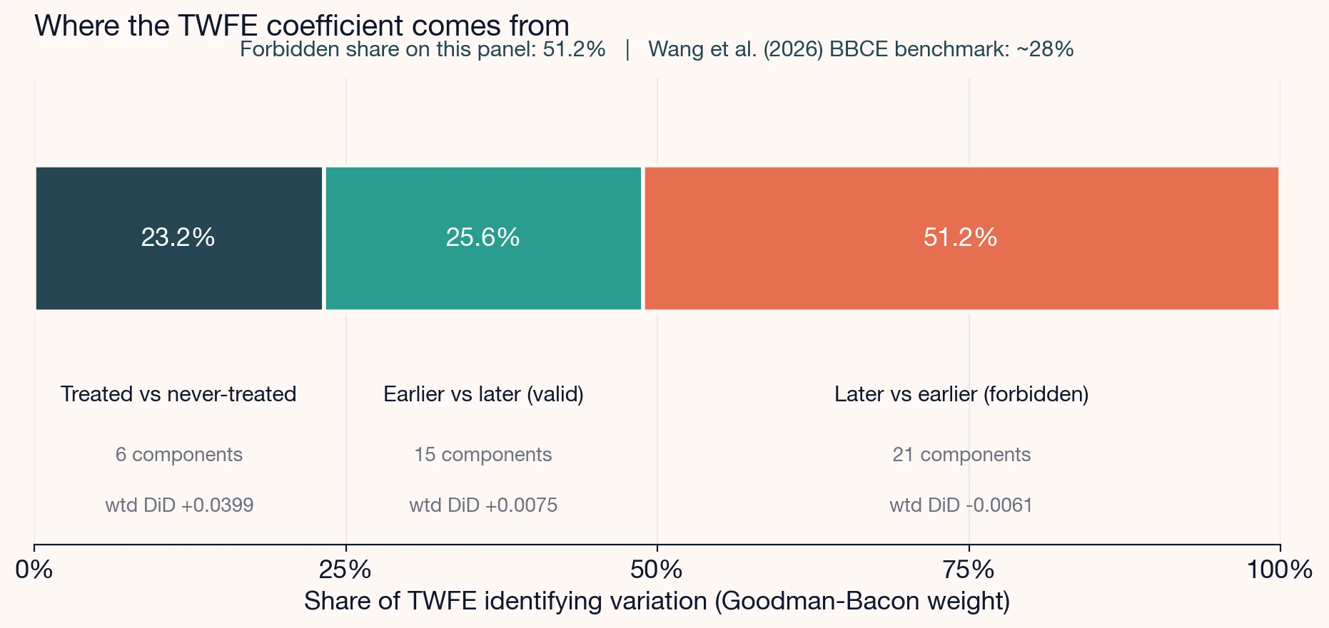
Goodman-Bacon decomposition of the two-way fixed-effects DiD estimator into its constituent 2x2 comparisons: treated vs never-treated weighted at 0.232 with mean effect 0.0399; earlier-treated vs later-treated (forward) weighted at 0.256 with mean effect 0.0075; later-treated vs earlier-treated (backward / forbidden) weighted at 0.512 with mean effect contribution -0.0061. The forbidden comparison carries the largest identifying-variation weight on this twelve-year panel.
The headline diagnostic here is the weight share on the forbidden row: 0.512. The reader-trap is to read this as "51% of my sample is doing forbidden comparisons." It is not. The weight is identifying-variation weight; a 2x2 comparison gets more weight when it spans more of the panel and when the treatment-timing happens closer to the middle of the observation window. Bacon's own framing: the weighted mean of the 42 components reproduces the TWFE coefficient. The weights tell us where the coefficient is coming from, not where the observations are.
What does 0.512 mean substantively? More than half of the TWFE coefficient on this panel is being built from comparisons that use already-treated units as controls for later-treated units. With heterogeneous treatment effects, those comparisons contaminate the estimate, and the direction of contamination depends on whether effects grow or shrink over time. The forbidden-component contribution here is -0.0061. The clean treated-vs-never component yields +0.0399, which is 9.7% of the pre-treatment baseline take-up rate. The forbidden component is pulling the headline estimate downward.
Wang et al. (2026) report the forbidden-comparison share for BBCE on their setting at approximately 0.28. Our 0.512 is nearly double their benchmark. Why?
The honest answer is sample window. Our panel is 2005-2016, twelve years. Wang's is 2000-2016, seventeen. A shorter window relative to treatment-timing variation means fewer never-treated comparison years, which mechanically raises the weight on later-vs-earlier-treated cells. We have not isolated this driver yet (a later part of the series will), but the direction is consistent with what the decomposition geometry would predict.
That higher forbidden share is itself a finding. It strengthens, rather than weakens, the case that the TWFE point estimate on this panel is the conservative bias-attenuated anchor in a two-estimator bracket. If TWFE on a longer panel understates the heterogeneity-robust estimator by 2x, TWFE on a shorter panel with a higher forbidden share would be expected to understate it by even more. The clean +0.0399 component is directionally aligned with Wang's CSDD upper bound of +15.3%, noting that the two estimates are on different outcome scales (the Part 2 Bacon component is on the take-up-rate outcome; Wang's CSDD is on log SNAP per capita).1 The contamination is bringing the headline down, not up.
Where the convergent evidence lands
Four diagnostics, one direction. The pre-period F-test rejects at p = 0.041 on one testable lead, with a small opposite-signed pre-coefficient that is not driving the headline estimate upward. The placebo test returns a statistical zero. The LOO is stable within ±6% across 41 iterations. The Bacon decomposition shows that 51% of the TWFE coefficient is forbidden-comparison contamination pulling the headline downward; the clean treated-vs-never component is +0.0399, directionally aligned with the heterogeneity-robust published benchmark.
What does this tell us? The marginal F-test failure on one lead is power-limited, not substantive. The convergent diagnostics (placebo at zero, LOO stable, Bacon contamination pulling the headline downward) together carry the credibility argument that a single low-power F-test cannot. The reading here is design-defensible rather than parallel-trends-verified, with the qualifier earned despite the marginal pre-test rejection with the explicit forward-link to Part 4 where the same panel gets re-estimated under Callaway-Sant'Anna and the parallel-trends question gets re-asked under the cohort-specific framework.4
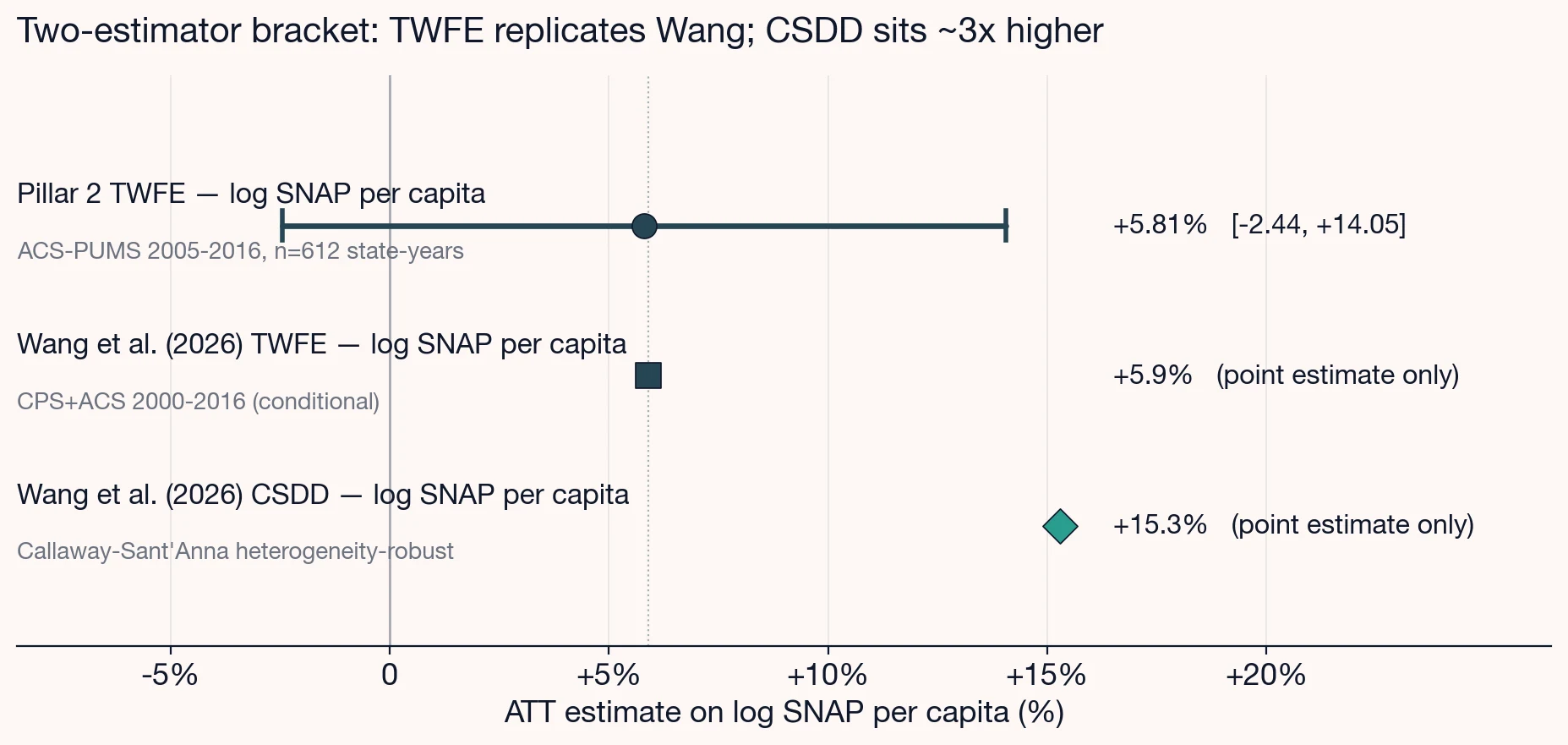
Forest plot of BBCE effect estimates on log SNAP per capita: Part 2 TWFE at plus 5.81 percent with a confidence interval spanning minus 2.44 to plus 14.05 percent; Wang et al. (2026) TWFE at plus 5.9 percent (near-exact match); Wang et al. (2026) CSDD heterogeneity-robust at plus 15.3 percent, roughly threefold larger and motivating the Part 4 forward-link to a heterogeneity-robust estimator.
Two further things this specification does not handle
The first is the BBCE-eligibility-expansion channel that the 130% FPL denominator does not absorb. The take-up-rate outcome identifies the take-up effect among the federally-eligible population, the 88.5% of the BBCE effect that does not come from extending eligibility to higher-income households. The other 11.5% is in Wang's log-pc specification and in Wang's eligibility-decomposition appendix, but it is not in our take-up-rate headline.1 A future robustness spec with a BBCE-adjusted denominator (130% FPL where BBCE is off, 200% FPL where BBCE is on) is deferred to Part 4.
The second is BBCE reversion. Two of the 41 ever-treated states drop BBCE in 2015 or 2016. The TWFE single-event setup conventionally assumes an absorbing-state binary (once treated, always treated). The specification here handles reversion with a time-varying treatment dummy: BBCE = 1 in the adoption-through-reversion years and BBCE = 0 elsewhere. Wang's specification handles BBCE the same way.1 The estimand under non-absorbing treatment is the average treatment effect on the treated while treated, and reverted-state post-reversion years contribute valid never-treated-equivalent observations to the comparison group. This is the canonical handling; we flag it for transparency but do not present it as a design flaw.
The defensible middle on TWFE
Why ship TWFE single-event at all in 2026, given that Wang and others document its contamination on this exact policy?
The honest defensible middle is that TWFE single-event is the canonical conservative bias-attenuated estimator. On staggered-adoption settings with heterogeneous treatment effects, TWFE understates the heterogeneity-robust target. Shipping TWFE alone, without disclosure, would mis-state the BBCE effect downward. Shipping the heterogeneity-robust upper bound alone, without TWFE, would lose the bracketing structure that lets a reader assess where the estimate sits in the literature. The defensible middle is to ship both with the contamination disclosure between them: TWFE here, heterogeneity-robust upper bound in Part 4, full Bacon decomposition between them so the reader can see exactly how much of the TWFE coefficient is forbidden-comparison weight and which direction it pulls.
TWFE remains a valid estimator when adoption is simultaneous across units and treatment effects are homogeneous. BBCE is neither. Adoption is staggered across 41 states over 2005-2011, and Wang et al. document on this exact policy that TWFE understates the heterogeneity-robust estimator by more than twofold. So we ship TWFE here as the lower-bound anchor in a two-estimator bracket. The recommended estimator for the BBCE policy question, the one we would want a referee to read as the headline number, lives in Part 4.
What this estimate is and is not
What we have on this panel is:
- A TWFE single-event ATT of +1.37 pp (+3.35% of baseline) on SNAP take-up among the federally-eligible, with the 95% CI overlapping zero (p = 0.18).
- A TWFE single-event ATT of +5.81% on log SNAP per capita, matching Wang's TWFE benchmark of +5.9% near-exactly on the same outcome.
- A pre-period F-test that rejects at p = 0.041 on a single testable lead, with the pre-coefficient signed opposite to the ATT.
- A placebo test at statistical zero (+0.78 pp, p = 0.37).
- A leave-one-out distribution stable within ±6% of the headline.
- A Bacon decomposition with 51% of the coefficient coming from forbidden comparisons that pull the headline downward, and a clean treated-vs-never component of +0.0399 (~9.7% of baseline) directionally aligned with Wang's heterogeneity-robust upper bound of +15.3%.
What this estimate is: a conservative bias-attenuated TWFE anchor on BBCE adoption, replicating Wang's TWFE log-pc benchmark near-exactly, with a full diagnostic stack and a transparent contamination disclosure.1
What this estimate is not: the recommended causal estimate of BBCE's effect on SNAP participation. That number lives in the heterogeneity-robust specification, which we hand off to Part 4 next.
The data suggests BBCE raised SNAP participation on this panel by +3.35% on the take-up rate outcome and by +5.81% on log SNAP per capita, with the true effect likely larger on both outcomes once the forbidden-comparison contamination is removed. The convergent diagnostics support that reading. The single-lead pre-test does not refute it. The two-estimator bracket lets the reader see exactly where the conservative anchor lands and where the heterogeneity-robust upper bound sits.
That is what we have. Next part, same panel, Callaway-Sant'Anna.
References
- Wang, X., Valizadeh, P., Nayga, R. M., Bryant, H. L., & Fischer, B. L. (2026). Broad-based categorical eligibility policy and SNAP participation. Journal of Policy Analysis and Management, 45(1), e70063. https://doi.org/10.1002/pam.70063
- Ganong, P., & Liebman, J. B. (2018). The decline, rebound, and further rise in SNAP enrollment: Disentangling business cycle fluctuations and policy changes. American Economic Journal: Economic Policy, 10(4), 153-176.
- Bertrand, M., Duflo, E., & Mullainathan, S. (2004). How much should we trust differences-in-differences estimates? The Quarterly Journal of Economics, 119(1), 249-275.
- Callaway, B., & Sant'Anna, P. H. C. (2021). Difference-in-differences with multiple time periods. Journal of Econometrics, 225(2), 200-230. https://doi.org/10.1016/j.jeconom.2020.12.001
- Roth, J. (2022). Pretest with caution: Event-study estimates after testing for parallel trends. American Economic Review: Insights, 4(3), 305-322.
- Goodman-Bacon, A. (2021). Difference-in-differences with variation in treatment timing. Journal of Econometrics, 225(2), 254-277. https://doi.org/10.1016/j.jeconom.2021.03.014