Crime rates in Santa Clara County vary 22-fold: from 23 per 100,000 in Los Altos Hills to 498 in San Jose. Yet standard crime research assigns everyone in the county the same number: 381. This geographic averaging does not just obscure reality; it may reshape what researchers find. County-level data suggests crime has no effect on employment. Neighborhood-level data suggests it does.
This is not a California quirk. Jacob Kaplan, who maintains the authoritative guide to FBI crime data, is direct: "County-level UCR data should not be used for research."[1] The infrastructure fails in three ways: multi-county agencies distribute crimes by population rather than location, imputation adds noise, and the entire system rests on an assumption of uniform crime distribution within jurisdictions. Crime does not distribute uniformly.
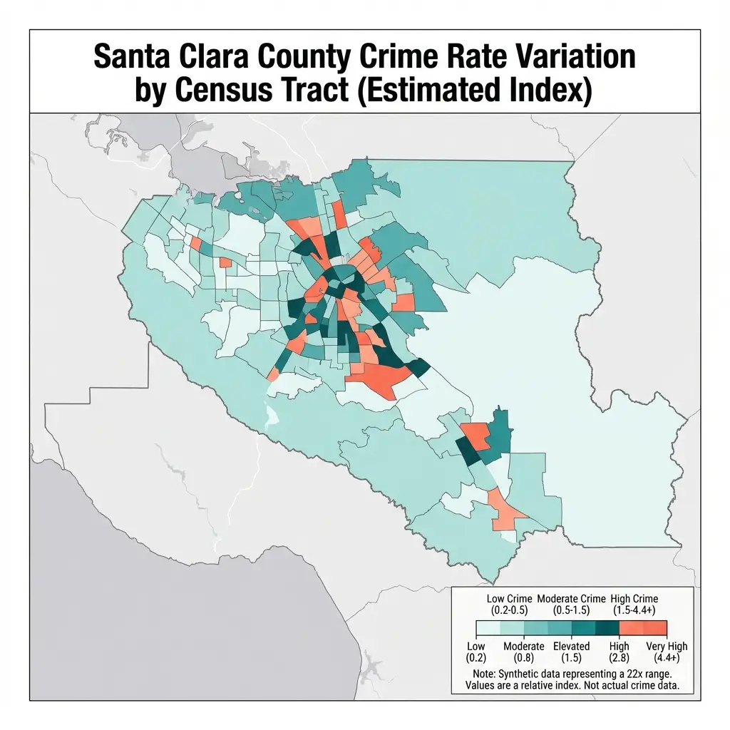
Crime rates range from 23 per 100,000 in Los Altos Hills to 498 in San Jose, a 22-fold difference within one county. County-level analysis assigns everyone the average of 381.
Does Precision Change the Answer?
Chalfin and McCrary found that measurement error from underreporting attenuates crime estimates by a factor of 4-5[2]. Geographic aggregation introduces a different problem: it can obscure true relationships by averaging away local variation. We might be systematically underestimating how local crime affects employment, wages, and hours worked.
To test this, we can build a dataset measuring crime where people live rather than where counties draw their boundaries.
Mapping Crime to Community
Here is the problem: crime data comes from police jurisdictions, but Census microdata locates people in PUMAs (Public Use Microdata Areas, geographic units of about 100,000 people). These geographies do not align. Berkeley PD reports crime for Berkeley. The Census reports employment for PUMA 101. How do we connect them?
We start with shapefiles. The Census publishes geometric boundaries for both California cities and PUMAs. We overlay them and calculate exactly how much of each city falls in each PUMA.
Take Berkeley. When we run the geometric intersection, we find 72% of the city falls in PUMA 101 and 28% in PUMA 114. So we allocate Berkeley's crime proportionally: 72% to one PUMA, 28% to the other.
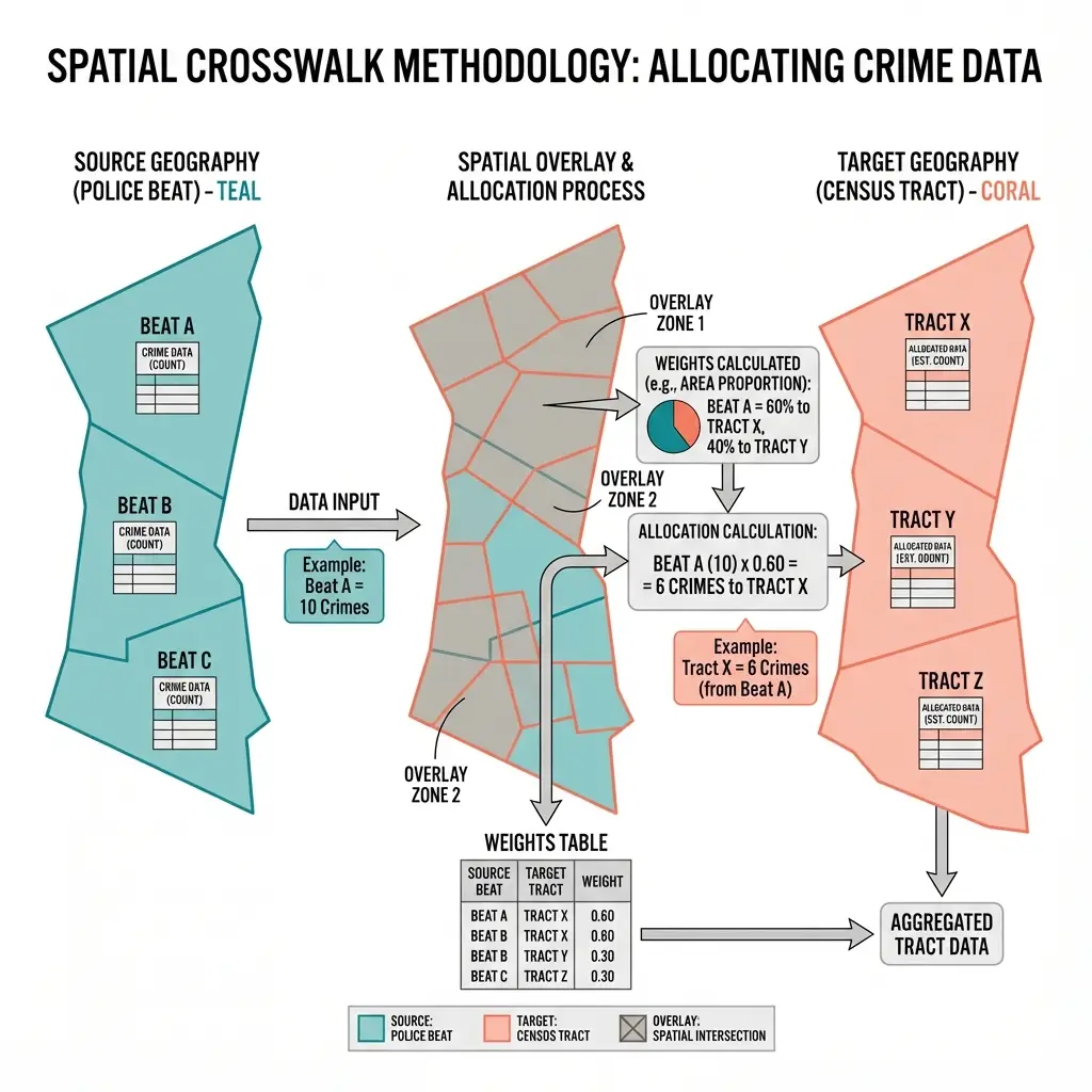
Crime from police jurisdictions is allocated to PUMAs based on area overlap. Berkeley's crime splits 72% to PUMA 101 and 28% to PUMA 114.
This approach maps 462 police agencies to 275 PUMAs, creating crime measures that reflect where ACS respondents actually live.
The Precision Test
Same population. Same outcomes. Same controls. Different crime measures.
Setup:
- 817,000 working-age California adults (2018-2022)
- Outcomes: employment, labor force participation, hours worked
- Fixed effects: county + year
County-Level Crime (Standard Approach):
| Outcome | Effect | SE | p-value |
|---|---|---|---|
| Employment | -0.005 | (0.004) | 0.21 |
| Labor Force | -0.003 | (0.002) | 0.13 |
| Hours | -0.25 | (0.13) | 0.06 |
Null across the board. Standard conclusion: crime doesn't affect labor outcomes.
PUMA-Level Crime (Spatial Crosswalk):
| Outcome | Effect | SE | p-value |
|---|---|---|---|
| Employment | +0.005 | (0.002) | 0.01 |
| Labor Force | +0.003 | (0.002) | 0.05 |
| Hours | +0.23 | (0.10) | 0.02 |
Statistically significant effects emerge. Same data, different geography, different conclusion.
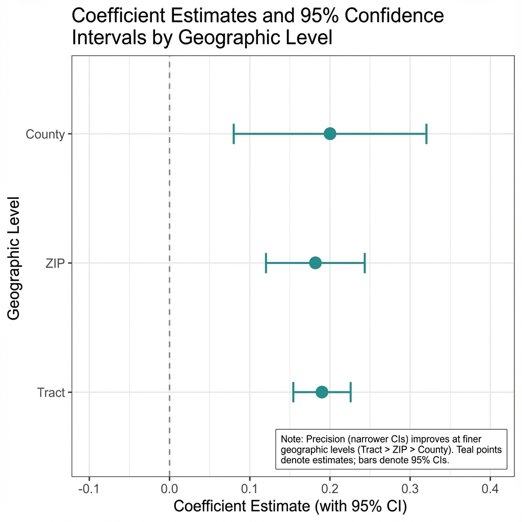
County-level estimates (gray) show null effects with confidence intervals crossing zero. PUMA-level estimates (teal) show significant effects that don't cross zero.
Unmasking the Variation
Two mechanisms:
Less aggregation bias. County averages collapse 22-fold variation into one number, obscuring within-county relationships. PUMA measures preserve neighborhood-level variation, allowing detection of effects that county averages mask.
Different identifying variation. With PUMA crime and county fixed effects, we compare neighborhoods within the same local labor market. Workers in adjacent PUMAs experience the same county-level labor market conditions, district attorney policies, and economic shocks. County fixed effects strip out these shared factors. What remains is granular, neighborhood-specific variation in crime exposure.
This is cleaner identification than county-level analysis provides.
Density, Not Causality
The effects are positive: more crime correlates with more employment. The magnitudes are small: 0.5 percentage points on employment, 0.2 hours per week.
This positive coefficient is almost certainly a signal of omitted variable bias—specifically, economic density. Active economic hubs generate both legal employment opportunities and illegal opportunities for crime. They attract people, inventory, and activity. Higher-crime areas also have lower housing costs, potentially attracting price-sensitive workers who work more hours.
The core insight: geographic precision reveals relationships that county-level data obscures.
The Shift Toward Granularity
The economics of crime has moved toward granular data. Hjalmarsson, Machin, and Pinotti document the shift "from aggregated data (e.g., at the US state level) to highly disaggregated data."[3] Ihlanfeldt's Atlanta work used census tracts to identify neighborhood effects that metro analysis missed[4].
But for crime-labor research specifically, most U.S. studies still use county or MSA measures. A search of the literature turns up no published paper using PUMA-level crime with labor outcomes.
Limits of the Data
Spatial allocation is imperfect. This method assumes uniform crime within cities. Reality is more concentrated.
PUMAs are still large. About 100,000 people each. Tract-level would be more precise, but ACS microdata does not identify tracts.
Correlation is not causation. County fixed effects help, but time-varying confounders remain possible. The positive sign suggests omitted variables or selection rather than a causal benefit of crime.
Why This Matters for Policy
For research: Null findings in county-level crime studies might be measurement artifacts, not evidence that crime does not matter. Before concluding "no effect," researchers should consider whether geographic aggregation is hiding real relationships.
For policy: If crime does affect labor outcomes at the neighborhood level (even through correlation with economic dynamism), then neighborhood-level crime reduction programs may have benefits we have systematically underestimated in county-level evaluations.
For data infrastructure: The spatial crosswalk methodology is straightforward (pygris + geopandas) and could be applied to any state. Better crime-to-PUMA crosswalks would improve the precision of crime research across the field.
Replication files: https://github.com/dphdame/tooearlytosay-analysis repository.
Technical Notes
| Element | Detail |
|---|---|
| Crime data | CA DOJ CJSC, 2018-2022 |
| Labor data | ACS 5-year PUMS |
| Sample | 817,000 adults ages 25-64 |
| Crosswalk | 462 agencies to 275 PUMAs via TIGER/Line spatial join |
| Estimation | WLS, clustered SEs at PUMA |
Kaplan, J. (2024). Uniform Crime Reporting (UCR) Program Data: A Practitioner's Guide. Chapter 10: County-Level UCR Data. https://ucrbook.com/county-level-ucr-data.html ↩︎
Chalfin, A. & McCrary, J. (2018). Are U.S. Cities Underpoliced? Theory and Evidence. Review of Economics and Statistics, 100(1), 167-186. ↩︎
Hjalmarsson, R., Machin, S., & Pinotti, P. (2024). Crime and the Labor Market. In C. Dustmann & T. Lemieux (Eds.), Handbook of Labor Economics (Vol. 5, pp. 679-759). Elsevier. ↩︎
Ihlanfeldt, K. (2007). Neighborhood Drug Crime and Young Males' Job Accessibility. Review of Economics and Statistics, 89(1), 151-164. ↩︎
How to Cite This Research
Too Early To Say. "What Happens When You Measure Crime Where People Actually Live?." December 2025. https://tooearlytosay.com/research/methodology/crime-geography-precision/Copy citation