Why Claude and ChatGPT Struggle with Research Graphics (And What Makes Antigravity Prompts Work)

Stack Overflow has accumulated 72,879 questions tagged matplotlib and another 57,712 tagged ggplot2. Reddit's r/dataisbeautiful (21 million subscribers) fields daily requests for help positioning legends, adjusting axis labels, and fixing overlapping annotations. The collective effort spent on research graphics is staggering, and much of it addresses the same fundamental problem: code can't see what it produces.

When we use Claude to generate Python visualizations, we often spend hours fighting a problem that shouldn't exist. A subtitle meant to clarify the chart renders behind the title. Callout boxes block the data points they're describing. Labels drift to corners instead of sitting where they'd be visually balanced.

Claude works fine. Python works fine. The gap is elsewhere: neither can see the output. The AI generates coordinates. The plotting library renders them mechanically. If something overlaps or looks wrong, nobody notices.

Google's Antigravity takes a different approach, and the results reveal both what AI image generation gets right and what researchers still need to verify themselves.

The Visual Reasoning Gap

When we ask Claude to create a coefficient plot, here's what happens:

1. The AI translates the request into matplotlib syntax
2. It specifies positions as numerical coordinates
3. The plotting library renders those coordinates exactly as specified
4. If something overlaps or looks unbalanced, nobody notices, because nobody can see

This is the visual reasoning gap. "Put the label on the right side, balanced with the left" becomes x=0.95, y=0.5, and neither Claude nor matplotlib knows whether that looks balanced. "Balanced" isn't a number. "Readable spacing" isn't a parameter.

Antigravity closes this gap. Google's tool uses Gemini's image generation model instead of writing code. Trained on images rather than syntax, it understands what "balanced" looks like, what "readable spacing" means, how elements should relate visually.

The difference shows up immediately.

Side-by-Side: Code vs. Antigravity

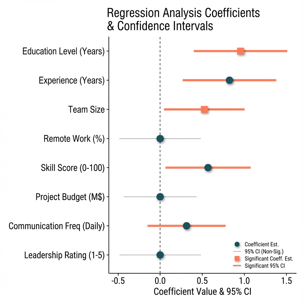
Coefficient Plot

Python output:

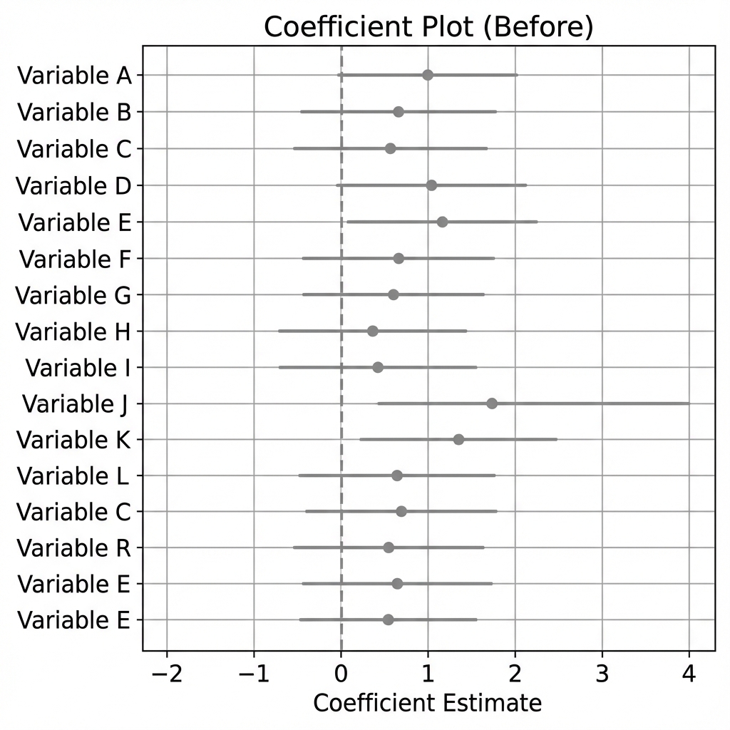
Antigravity output:

Icon Array

Python output:

Antigravity output:

Choropleth Map

Stata output (after 2 hours of debugging):

To be fair: spmap has worked in the past, always after a surprisingly long debugging session. Whether it's user error at this point, hard to say. But given the alternatives, it's not something worth worrying about. Even without generative AI, Python handles the same task in under 10 lines with native GeoJSON support. Stata excels at statistical graphics; for geographic visualization, there are easier paths.

Antigravity output:

Causal Diagram (DAG)

What Makes an Antigravity Prompt Work

Vague prompts produce vague results. The difference between frustration and a usable output comes down to structure.

The Coefficient Plot Prompt

Create a coefficient plot showing four predictors of food vulnerability:
poverty rate, SNAP enrollment, vehicle access, and transit time.

Include 95% confidence intervals as horizontal lines through each point.
Add a vertical dashed line at zero.

Use these approximate values:
- Poverty Rate: 0.42 (CI: 0.28 to 0.58)
- SNAP Enrollment: 0.31 (CI: 0.18 to 0.45)
- No Vehicle Access: 0.19 (CI: 0.08 to 0.29)
- Transit Time (min): 0.08 (CI: 0.02 to 0.14)

Title: "Predictors of Food Vulnerability"
Subtitle: "Coefficient Estimates with 95% Confidence Intervals"
Source note: "Food Security Analysis, 408 census tracts"

Use a clean, publication-ready style with readable axis labels.

Why this works:

• Visualization type ("coefficient plot") — Anchors the request in a known format
• Exact values with CIs — Enables verification; no hallucinated numbers
• Structural elements ("dashed line at zero") — Specifies conventions the AI might omit
• All text content — Nothing left to imagination

The key insight: provide the data explicitly. Stating the values ensures accuracy and enables verification.

The Icon Array Prompt

The data here comes from our transit accessibility analysis, which found that 1 in 8 California neighborhoods have grocery stores nearby but lack transit access to reach them.

Create an icon array showing that 1 in 8 households in Santa Clara County
lives more than 45 minutes from a grocery store by transit.

Show a grid of 24 rounded squares arranged in 3 rows of 8.
Highlight 3 squares in red (#dc2626), leave 21 squares in light gray (#e5e7eb).

Title: "In Santa Clara County..."
Subtitle: "1 in 8 households lives more than 45 minutes
from a grocery store by transit"

Legend at bottom:
- Red square = "45+ min to groceries"
- Gray square = "Under 45 min"
- Note: "Each square represents ~5,000 households"

Why this works:

• Grid dimensions ("3 rows of 8") — Prevents wrong proportions
• Exact count ("3 highlighted") — Mathematically correct (3/24 = 1/8)
• Hex colors (#dc2626) — Precise control; "red" is ambiguous

The Choropleth Prompt

Create a choropleth map of Santa Clara County, California
showing food vulnerability by census tract.

Use a blue color scale (light = low, dark = high) with 5 quantile breaks.

Show the characteristic shape of Santa Clara County: urban areas
in the north (San Jose, Sunnyvale) and rural areas in the south.

Title: "Food Vulnerability by Census Tract"
Legend: "Vulnerability Score" with 5 color gradations
Source note: "Higher values = greater vulnerability"

Clean white background, no basemap clutter.

Why this works:

• Geographic context (city names) — Helps AI render recognizable shape
• Color scale direction ("light = low") — Prevents inverted interpretation
• Negative instruction ("no basemap clutter") — Removes unwanted elements

The Five Rules for Effective Prompts

1. Name the visualization type. "Coefficient plot," not "a chart showing regression results."
2. Provide exact values. Don't hope Antigravity reads your data correctly. State the numbers.
3. Specify colors with hex codes. "Blue" is ambiguous. #2563eb is precise.
4. Include all text. Titles, subtitles, axis labels, legend entries, source notes. Everything.
5. State what you don't want. "No gridlines," "white background." Negative instructions prevent clutter.

The Verification Imperative

Here's the catch: we can only outsource what we can verify.

When Antigravity generates a coefficient plot, how do we know the point estimates are plotted at the correct values? That the confidence intervals are the right width? That the scale is accurate?

With code, we can trace the pipeline: data → transformation → plot command → output. With Antigravity, there's a black box between the prompt and the result.

Three verification approaches:

1. Cross-check against code output. Generate a rough version in R first. It doesn't need to look good; it needs to be verifiably correct. Then use Antigravity for polish, comparing against the baseline.

2. Request explicit data labels. Prompt the tool to label each point with its value: "Label each coefficient with its point estimate and confidence interval." Now you can visually verify each number.

3. Use AI for styling only. Feed it your verified plot and ask it to "make this publication-ready while preserving all data points exactly."

The approach depends on the graphic type. For coefficient plots with precise numerical claims, always verify. For icon arrays showing "1 in 8 households," verification is simpler: count the highlighted squares. For conceptual diagrams like DAGs, there's no numerical precision to verify, just logical relationships.

When Code Still Wins

Antigravity doesn't replace code for everything:

Reproducibility. If you need to regenerate the same figure with updated data, code wins. Antigravity may produce slightly different results across sessions.

Automation. If you're generating 50 county-level maps programmatically, code wins. Antigravity is conversational, great for single outputs but inefficient for batch processing.

Iteration. When you're still exploring and don't know what the final graphic should look like, quick-and-dirty code output helps you think. Save Antigravity for when decisions are settled.

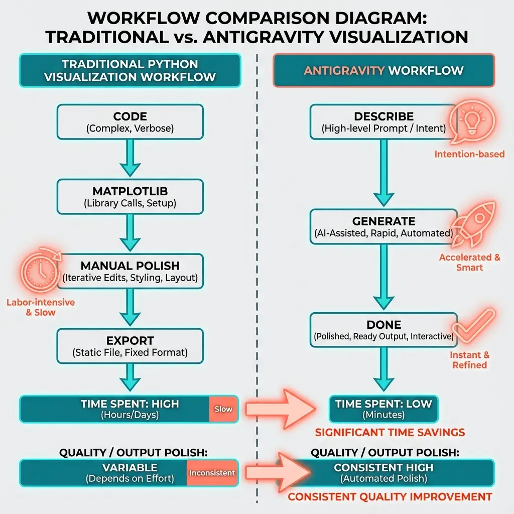
The Hybrid Workflow

In practice, we use multiple tools:

1. R/Python for iterating on design choices (free, reproducible)
2. R/Python for verification baseline (verifiably correct)
3. Antigravity for final publication-ready version (visually polished)

The traditional tools handle exploration cheaply. Antigravity produces the polished final output. This minimizes cost while maximizing quality.

Claude and ChatGPT write code that can't see. Antigravity makes images that can. For research graphics, knowing when to use each, and always verifying, is what makes the workflow trustworthy.

Prompts and Code: Example prompts and comparison code available by request. Contact [email protected].

Citation

Cholette, V. (2025, December 19). Why Claude and ChatGPT struggle with research graphics (and what makes Antigravity prompts work). Too Early to Say. https://www.tooearlytosay.com/ai-research-graphics-antigravity/